Clustering#
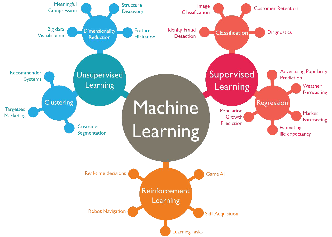
Unsupervised Learning#
Dimensionality Reduction
reducing dimension of feature space by finding informative feature representations (for ML algorithms or humans)
visualization in 2D
Clustering
grouping similar samples
# Warm-up: Try to find pairs (using ipython, e.g.)
# CAVEAT: requires some research!
left = [
'Outlier or anomaly detection can be used',
'Principal Component Analysis (PCA) is a method',
'Principal Component Analysis (PCA) is frequently used',
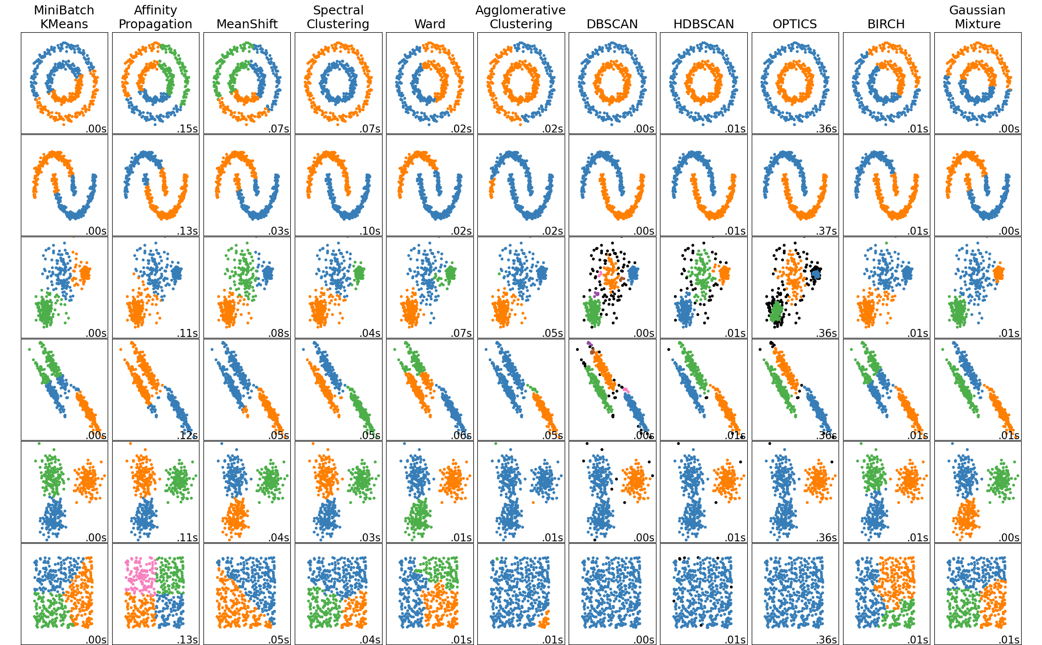
'There are many clustering methods',
'Most clustering algorithms are based on a distance metric',
'Gaussian Mixture Models (GMM) are a generative model',
'Unsupervised learning is a family of machine learning methods',
'The "curse of dimensionality" is a problem',
't-SNE reduces data to two dimensions'
]
right = [
'to visualize complex datasets.',
'that becomes worse the more features you have.',
'to identify credit card fraud.',
'for dimensionality reduction.',
'e.g. Euclidean or Manhatten distance.',
'that do not require labled data.',
'for detecting outliers.',
'as part of a supervised learning pipeline.',
'like K-means, agglomeration, or DBSCAN.'
]
Clustering#
Idea: Partition the dataset into groups (clusters) so that
observations in same cluster are as similar as possible
observations in different clusters are as different as possible
application examples
anomaly detection (e.g. fraud detection, technical maintenance)
recommender systems (e.g. literature/movie/cloth recommendations)
no personalized but groupwise patient treatments (e.g. rehabilitation programs)
…
Similarity Measures#
The distance between two points \(a_1\) and \(a_2\) in n-dimensional space
can be measured in different ways:
Euclidean distance (“length” of connecting line)
Manhattan distance (taxicab distance)
Minkowski distance (generalisation of above distance metrics)
Cosine similarity (cosine of the enclosed angle)
The similarity of sets A and B can be measured by the Jaccard index
…
\( d_{Eucl}(a_1,a_2) = \sqrt{(a_2-a_1)^2} \)
\( d_{Manhattan}(a_1,a_2) = \sum_{i=1}^n \left|a_{2,i} - a_{1,i}\right|\)
\( d_{Mink}(a_1,a_2) = \biggl(\sum_{i=1}^n |a_{2,i}-a_{1,i}|^k\biggr)^{\frac{1}{k}}\)
\( d_{cosine}(a_1,a_2) = {a_1 \cdot a_2 \over {\|a_1\| \|a_2\|}}\)
\( J(A,B) = \frac{|A \cap B|}{|A \cup B|} \)
Application examples for DS purposes#
convenient inspection of single clusters (instead of the complete dataset, e.g. for visualisations)
create groups as features or outcomes for predictive regression or classification model
create pseudo-labels for semi-supervised learning
K-Means clustering#
Idea of K-means#
Define the number of clusters, k (hyperparameter).
Assign all observations to a certain cluster so that within-cluster distances (hyperparameter) are minimal.
Cluster mean does not refer to a single number, but to the n-dimensional means of all features.
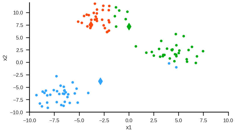
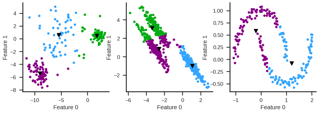
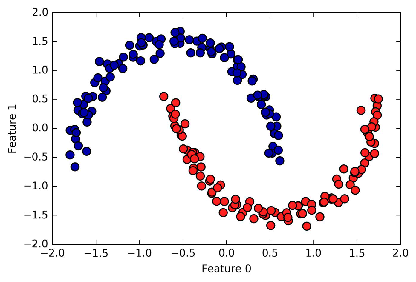
Example#
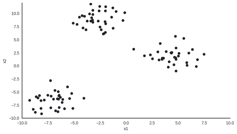
Sample with two features x1 and x2, 100 observations and obviously 3 clusters.
Example#
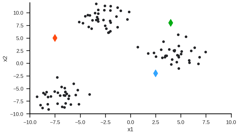
Step 0: Randomly initialize (or user-define) starting cluster centroids.
Step 1: Assign observations to closest cluster centroid (initial/new clusters).
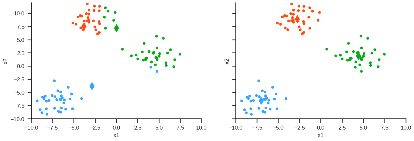
Example#
Step 2: For each cluster (here: red, green, blue) calculate the mean values for each of the features (here: x2 and x1). These mean values are the coordinates of the new cluster centroids:
Example#
Step 3: Repeat from Step 1 (reassign points) until the following sum is minimised:
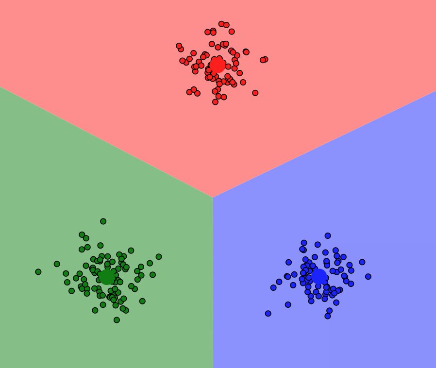
K-means in action#
To see K-Means in action, check out this amazing blog by Naftali Harris.
How to find the best number of clusters?#
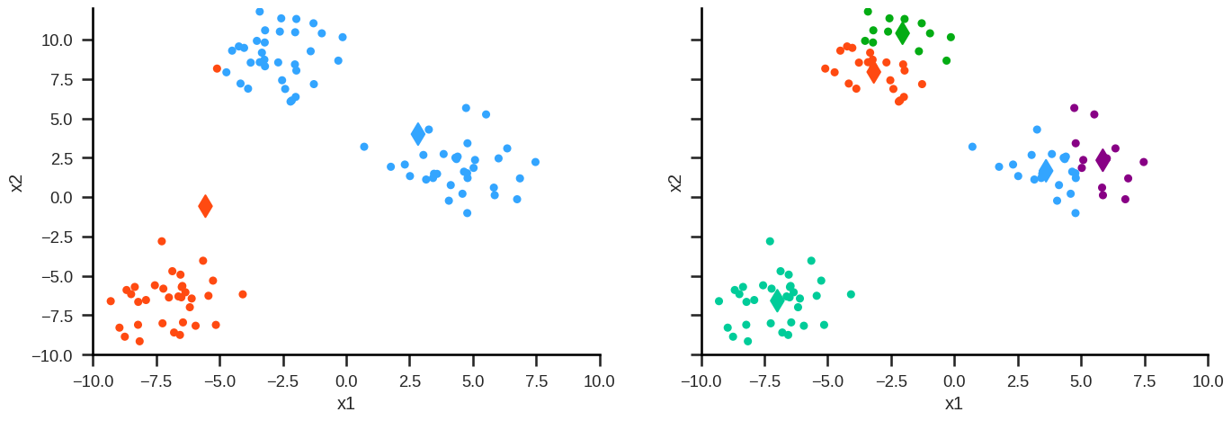
Elbow Method#
test different amount of clusters k
→ k is a hyperparametercalculate performance metric (eg. within-cluster sum of squares)
decide for the amount of clusters where an additional cluster contributes only marginally
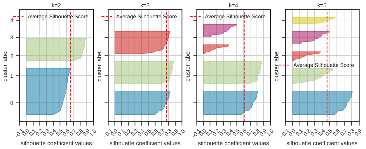
Silhouette plot and silhouette coefficients#
The Silhouette score measures how well each data point fits within its assigned cluster compared to other clusters.
Silhouette plot:
based on silhouette coefficients (cluster average score) and score
“knives” should extend over dashed line
similar sizes are preferable
Silhouette coefficients:
close to 1: good clustering
close to 0: overlapping clusters
close to -1: incorrectly assigned
K-means considerations#
Pros
fast (computational effort scales with size of dataset, viz. linear)
simple and therefore understandable
interpretable results (e.g. centroid can be regarded as characteristic for a cluster)
Number of clusters can be defined (advantageous if specified by the business case)
Cons
Cannot easily handle clusters with different diameters,
nor non-convex clusters.
Number of clusters has to be defined (hyperparameter)
K-means considerations#
General
Scale variables before clustering otherwise variables with large scale will dominate the clustering process.
K-means does not care for a balance within a dataset.
It’s a greedy algorithm with outcome depending on initialization.
Improvements
k-means++ (tends to select centroids that are distant from one another)
Balanced K-means (enforces the cluster sizes to be strictly balanced)
Regularized K-means (effective clustering of high-dimensional data)
Hierarchical clustering#
Idea#
Finding clusters not depending on random initialization.
Agglomerative algorithm#
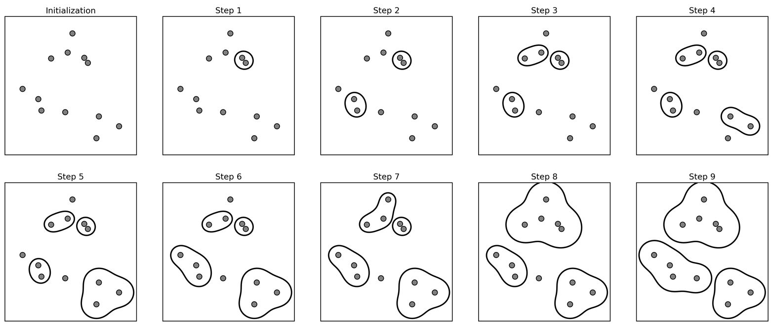
Visualization#
Dendrogram:
Visual representation of records and hierarchy of clusters to which they belong
(“dendro” is greek for tree)
Visualization#
plotting Dendrogram (visualize hierarchical clustering)
samples are numbered
shows order in which samples are clustered together (reading from bottom to top)
y-axis shows how far apart clusters are
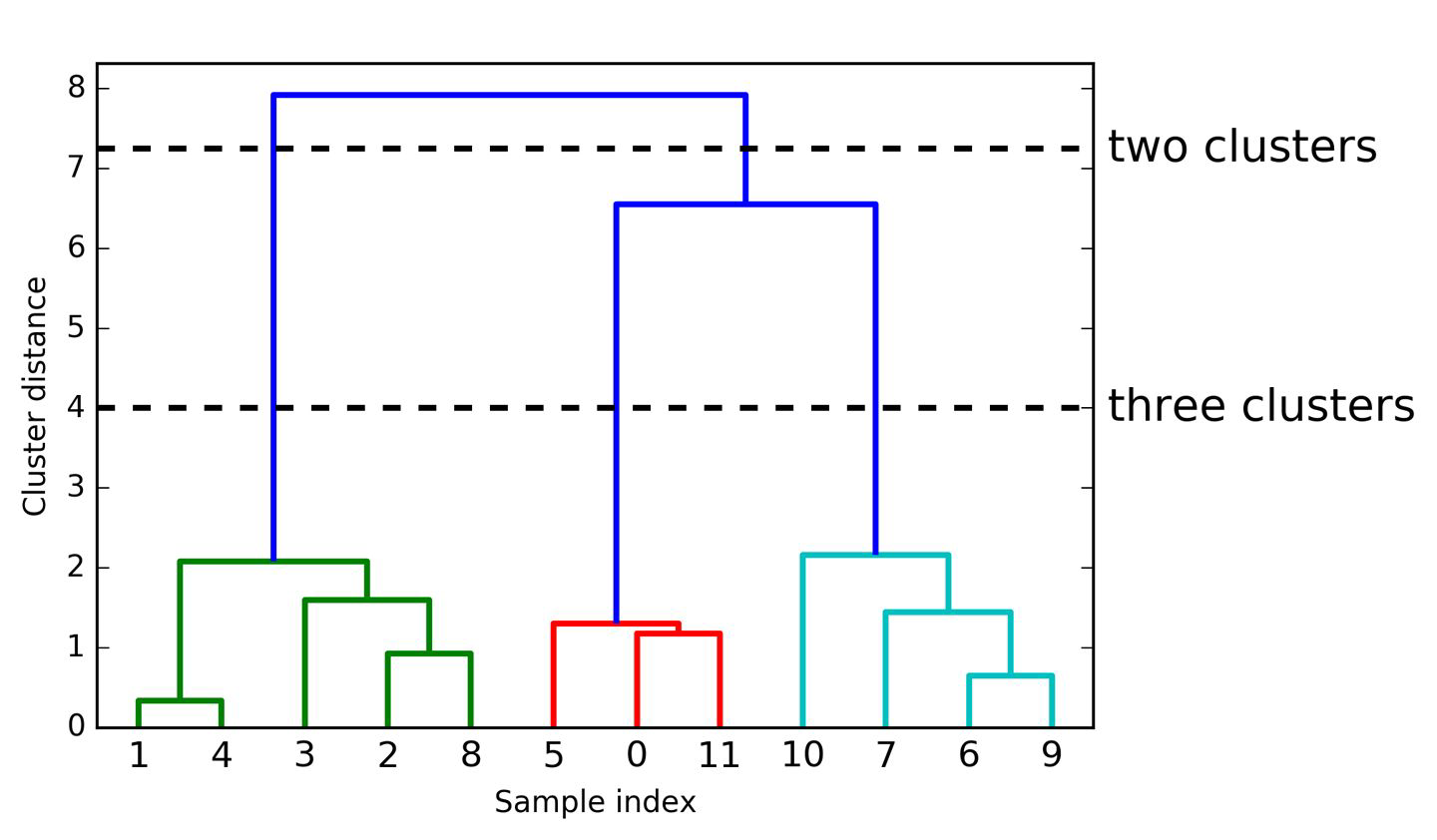
How to find the best number of clusters?#
plotting Dendrogram (visualize hierarchical clustering)
samples are numbered
shows order in which samples are clustered together (reading from bottom to top)
y-axis shows how far apart clusters are
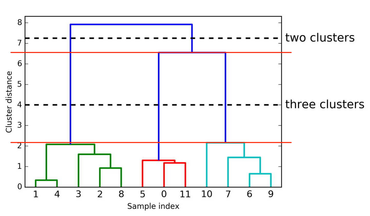
→ optimal number of clusters: largest vertical distance within same number of clusters
Dissimilarity Metrics#
We need to define how far two observations / clusters are away from each other
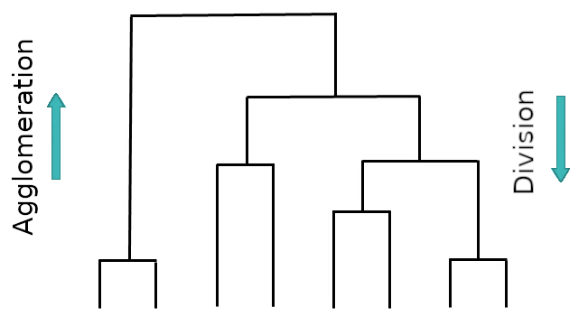
Bottom up vs. top down#
So far we investigated agglomeration (bottom up)
Alternatively there is also divisive clustering (top down)
Drawbacks of Agglomerative Clustering#
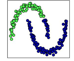
not able to capture complex structure
does not scale well with large data sets
greedy algorithm (might not be globally optimal)
DBSCAN#
Idea#
DBSCAN: Density-based spatial clustering of applications with noise
Idea:
clusters dense regions which are separated by areas that are relatively empty
it identifies points that don’t belong to any cluster (aka noise)
Two hyper-parameters#
eps (max distance considered between points of a cluster)
min_samples (required to form a cluster)
The core point itself is also counted when checking the min_samples requirement.
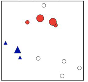
Three types of points#
Core point:
if there are at least min_sample points within distance eps
Three types of points#
Core point:
if there are at least min_sample points within distance eps
Boundary point:
if there is at least one core point within distance eps
but less neighbouring points than min_samples
Three types of points#
Core point:
if there are at least min_sample points within distance eps
Boundary point:
if there is at least one core point within distance eps
but less neighbouring points than min_samples
Noise (outlier):
if neither core nor boundary point
→ not reachable from any other cluster
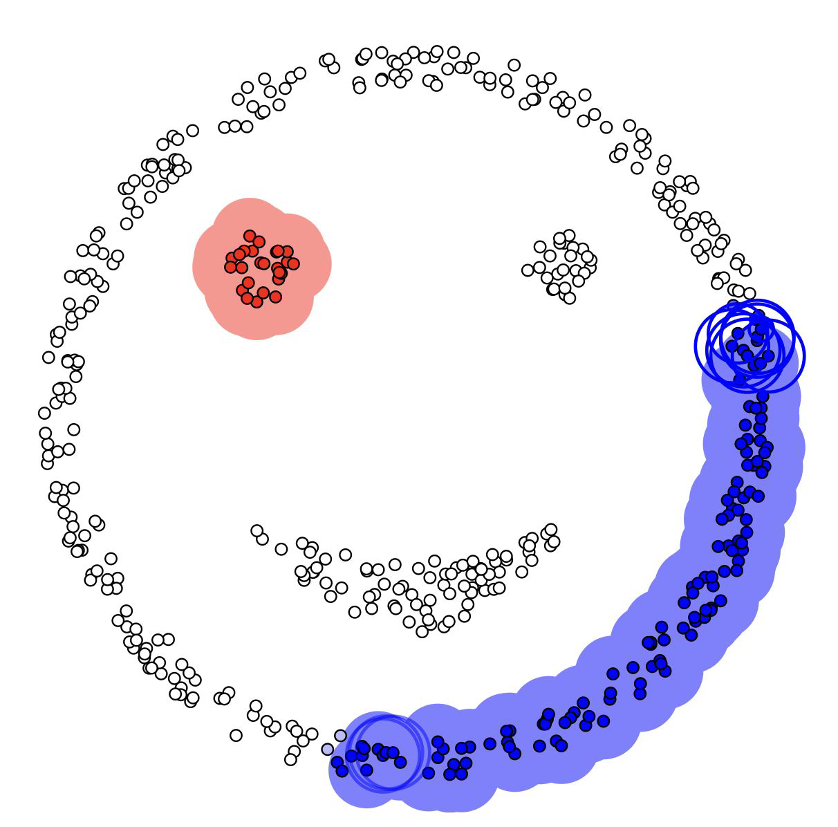
Procedure#
Advantages#
automatically identifies number of clusters
able to identify complex formed clusters
able to identify clusters with very different sizes
distinguish between clusters (dense data) and noise
However, boundary points can belong to different clusters. DBSCAN assigns those arbitrarily to one possible cluster.
DBSCAN in action#
To try out more DBSCAN in action, check out this amazing blog by Naftali Harris.
Summary#
Great documentation page on scikit-learn!