Bias Variance Tradeoff

Let’s start with IceCream

Let’s start with IceCream

Visual Approach

Why is it necessary to split the data into train and test?

Data is typically split into a train and a test set.

• to evaluate how the model performs on unseen data
  i.e. if the model ‘generalises’ well

• typical splits are 70% train data (or more) and 30% test data (or less)

• sometimes an additional validation set is used

Read more on splitting

Simple Model

Complex Model

Train Data Residuals

Test Data Residuals

Machine Learning Terminology

Too simple model:

• high bias

• under-fits the data

• low variance

• generalizes better on new data

Too complex model:

• low bias

• over-fits the data

• high variance

• generalizes bad on new data

Machine Learning Terminology

Too simple model:

• high bias

• under-fits the data

• low variance

• generalizes better on new data

Too complex model:

• low bias

• over-fits the data

• high variance

• generalizes bad on new data

Loss and Cost functions

Loss function

The loss function quantifies how much a model \(f\)‘s prediction \(\hat{y}=f(x)\) deviates from the ground truth \(y=y(x)\) for one particular object \(\mathbf{x}\).

So, when we calculate loss, we do it for a single object in the training or test sets. There are many different loss functions we can choose from, and each has its advantages and shortcomings. In general, any distance metric defined over the space of target values can act as a loss function.

Cost function

The cost function measures the model’s error on a group of objects. So, if L is our loss function, then we calculate the cost function by aggregating the loss L over the training, validation, or test data.

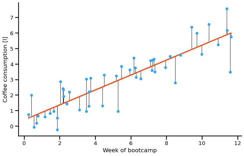
Linear Regression

MSE (mean squared errors) here is an example of a cost function - we’ve aggregated the loss of individual predictions into a single value we can use to gauge the quality of our model.

\[\begin{split}\begin{align} \hat{y} &= b_{0}+b_{1}x_{1}+\text{...}+b_{m}x_{m}\\[8pt] e &= y-\hat{y}\\[12pt] \text{MSE} &= {\frac{1}{n}}\sum_{i=1}^{n}{(y_{i}-{\hat{y}}_{i})}^{2} \end{align}\end{split}\]

Optimal model and prediction for linear regression

\[\begin{split}\begin{align} y&=f(x)=\beta_{0}+\beta_{1}x+\epsilon \\[5pt] \hat{y} &= b_{0}+b_{1}x_{1}+\text{...}+b_{m}x_{m} \end{align}\end{split}\]

In frequentist statistics, we make a point estimate of beta depending on the dataset D

Estimators

Assumption for estimators

• Dependent on the data:
  Different datasets give different estimation values
  
  \[\hat{y}(x,\;{\cal D})\;\;\;\;\;{\cal D}=\{\left(x_{1},\;y_{1}\right), \text{...}, (x_{n},\;y_{n})\}\]
• Data is randomly sampled
  No obvious patterns
  
• Parameters are considered to be fixed
  Data Generating Process (DGP):
  \[y=f(x)=\beta_{0}+\beta_{1}x+\epsilon\]

Estimates

• We rarely have money/resources to measure everything

• So we will have samples of the population which we hope to be representative of the whole population

• The more data we have the more confident we are in the estimates

• Ideally: the results drawn from our experiments are reproducible

In Data Science most metrics omit the word “estimate”, nevertheless most of the metrics we use are estimates

Error Decomposition

\[Bias^2 + Variance + Noise\]

\[\underbrace{Bias^2}_{underfitting} + \underbrace{Variance}_{overfitting} + \underbrace{Noise}_{unpredictable}\]

Bias

Bias: simplifying assumptions made by a model to make the target function easier to learn. (“How far away are the decisions from the data.”)

• Underfitting the training data

• Making assumptions without caring about the data

• Model is not complex enough

Linear algorithms tend to have high bias, this makes them fast to learn and easier to understand but less flexible.

Variance

Variance is the amount that the estimate of the target will change if different training data was used.

How sensitive is the algorithm to the specific training data used.

• Overfitting the training data

• Being extremely perceptive of the training data

• Model is too complex

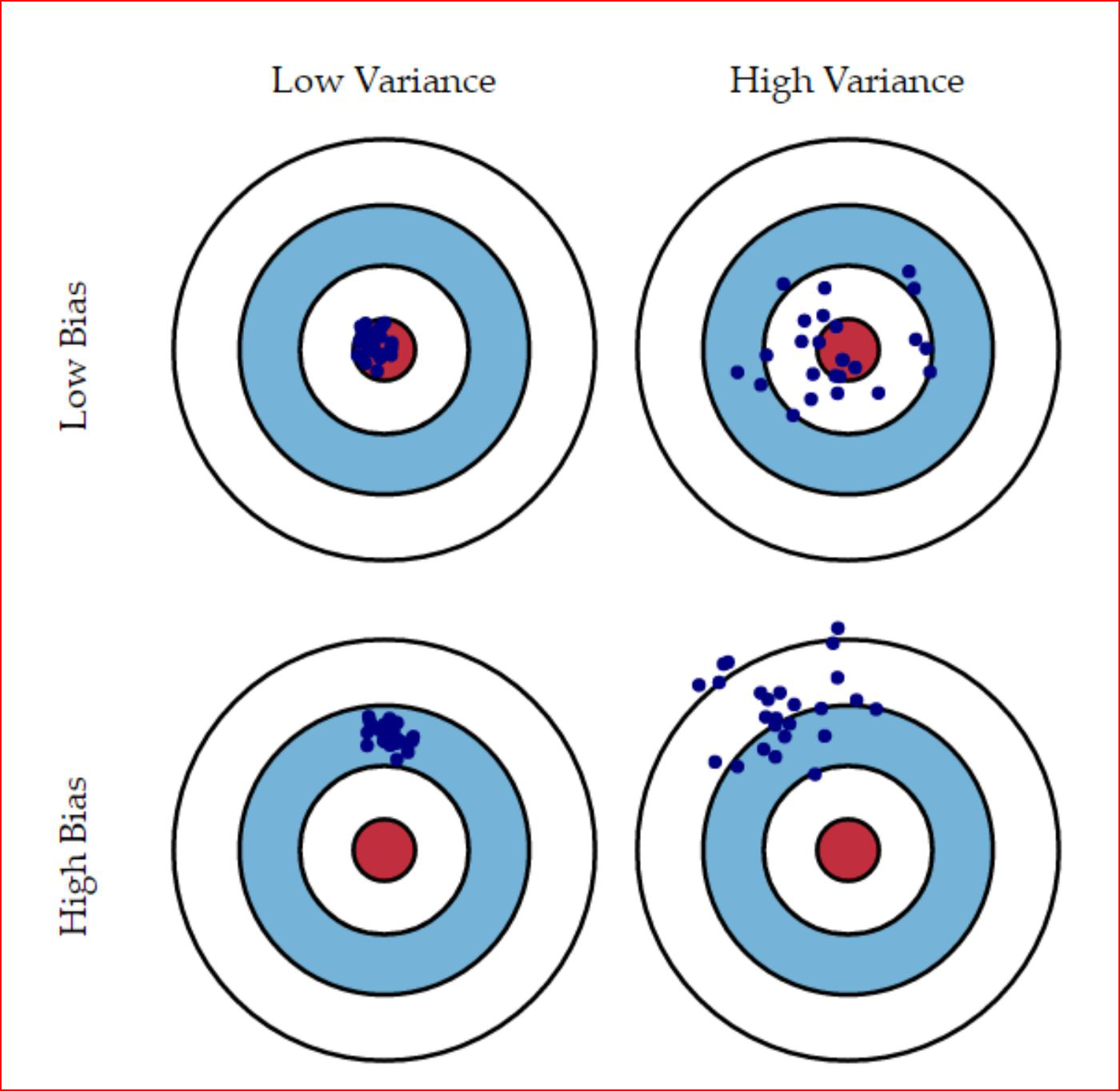
The Bias-Variance-Tradeoff

\[\frac{d\,Bias^{2}}{d\,Complexity}=-\frac{d\,Variance}{d\,Complexity}\]

Bulls-eye - a model that predicts perfectly

Do you want a clock that is sometimes 10 mins late or a clock that is always 10 mins late?

Desirable properties of estimators

Minimum variance estimators

• Prevent overfitting

Unbiased estimators

• Prevent underfitting

A model as simple as possible

“A simple model is the best model” - Occam’s Razor

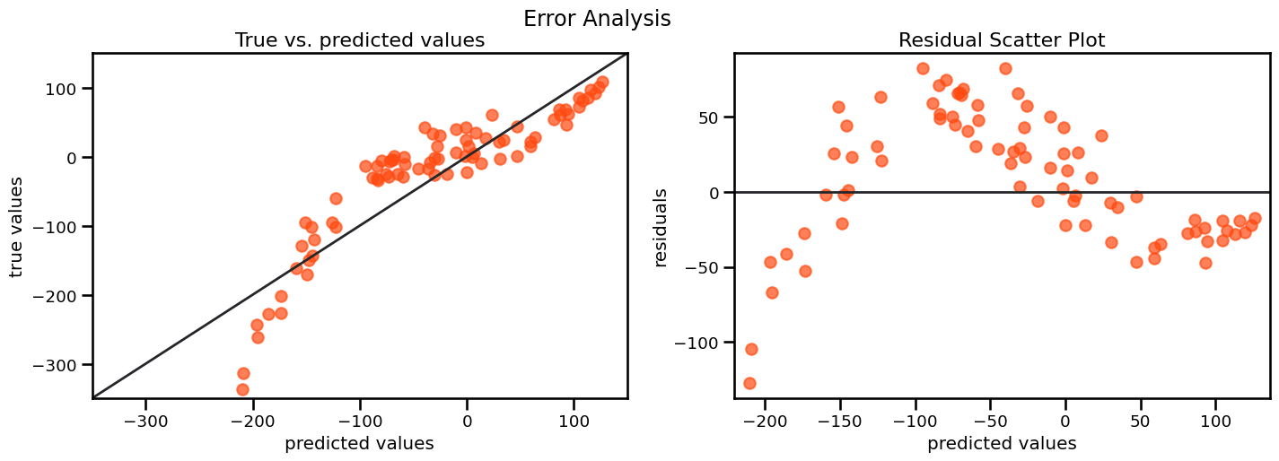
Error Analysis

The EDA for the errors your model makes

• comparing the errors on test / train / validation

  • expecting them to be close

  • low error on train but high on validation is a clear sign of overfitting

• plotting residuals

  • expecting no pattern

  • pattern in residual plots are a sign for underfitting => your model is not complex enough

Analyzing residuals

error_analysis(*lin_reg_model_for_error_analysis())

Bias vs. Variance

High Bias:

more assumptions of the target function

• Linear Regression, Logistic Regression

High Variance:

large changes to the estimate when train data changed

• Decision Trees, K-Nearest Neighbors …

Low Bias:

fewer assumptions about the target function

• Decision Trees, K-Nearest Neighbors, …

Low Variance:

small changes to the estimate when the train data changes

• Linear Regression, Logistic Regression

Overfitting vs. Underfitting

Overfitting:

• Reduce the complexity of the model

• Get more data

• Regularize the model

Underfitting:

• Bring in a better model

• Feature engineering

• Ease regularization parameters

Can you solve this little riddle?

\[\begin{split}\begin{align} f(1)&=1 \\ f(2)&=3 \\ f(3)&=5 \\ f(4)&=7 \\ f(5)&=??? \\ \end{align}\end{split}\]

It’s obvious, isn’t it?

\[f(5)=217341\]

At least if you apply this function

\[ f(x)=\frac{1811}{2}x^{4}-90555x^{3}+\frac{633885}{2}x^{2}-452773x+217331\]

This is a nice example taken from University of Berkeley to showcase how you can under do it when it comes to fitting a model.

What kind of error have you done with your personal model?

Resources

Hands-on ML with scikit-learn and TensorFlow, Geron, Geron

http://scott.fortmann-roe.com/docs/BiasVariance.html

https://medium.com/analytics-vidhya/bias-variance-tradeoff-for-dummies-9f13147ab7d0

Machine Learning - A probabilistic Perspective - Kevin P. Murphy

https://explained.ai/regularization/constraints.html

https://explained.ai/statspeak/index.html