Image Modeling#
Warm-up 🌶️#
Spend some time looking at this explanation of Image Kernels (feel free to play around with all the settings!) and discuss the following questions:
What does the number at each pixel location in a greyscale image mean?
What is a kernel?
How is a kernel applied to an image?
How does changing the numbers in the kernel affect the output image?
What features of an image can we highlight using a kernel?
Motivation#
Image Data#
There is possibly no other data that has increased as much over the last decade - and filled our everyday life - as image data
In a single day on Instagram 1.3 billion photos and videos are uploaded (2023)
We want to process such data for many reasons
Image classification and captioning
Toxic content detection
Image quality improvements, etc.
Introduction#
How does image data look like?#
Image data has height, width and depth
Height and width are given in pixels
Depth is the number of channels (3 for RedGreenBlue, 1 for BlackWhite)
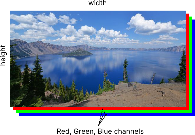
Each pixel corresponds to an integer between 0 and 255
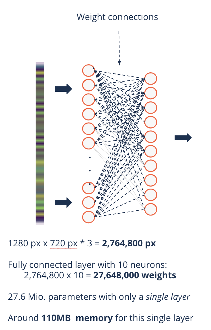
Example: A 1280 x 720 px color image has 1280 x 720 x 3 = 2,764,800 pixels = 2.76 MB
That is a lot to digest for an ML model using thousands of images for training and maybe hundreds in a batch
Unstructured data and locality#
In contrast to structured table data images show regularly transformations in local features
Different angles, rotations, flipping, scaling, translations
Humans can see the same objects just naturally
For an ML model this is a challenge
Transformation invariance is desired
Principle of locality#
Nearby pixels often show the same or a similar color
As pixels become further apart this similarity decreases or even breaks
Locality describes this phenomenon:
Locally pixels are correlated
Structured and unstructured data#
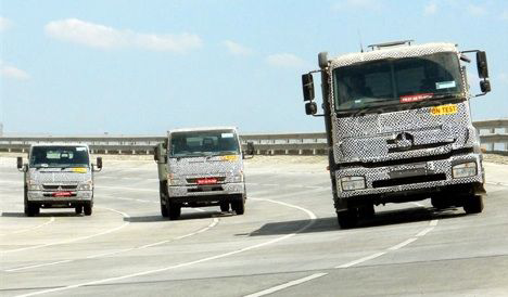
With structured data we would simply compare two feature vectors
Example: Structured truck data
Structured and unstructured data#
With structured data we would simply compare two feature vectors
Example: Structured truck data
Comparing the euclidean distance:
\((2.849-2.420)^{2}+(28-11)^{2}=289.19\)
\((2.975-2.420)^{2}+(50-11)^{2}=1,521.31\)
Structured and unstructured data#
With structured data we would simply compare two feature vectors
Example: Structured truck data
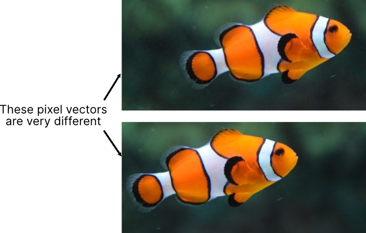
This does not work with image data comparing the vectors of all pixels (rolling them out)
The reason is locality (more generally transformation)
What is ideal feature information?#
The primary information to identify objects in an image are the pixel relations
Pixels distributed in a certain way identify a certain object
Colour compositions play in certain areas a crucial role
But how can we extract features that contain this information from an image?
This is a demanding task
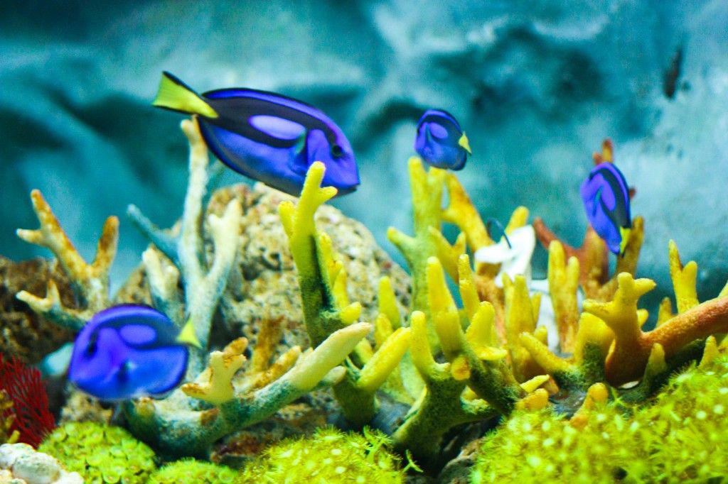
How do we humans identify a fish as a fish?
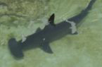
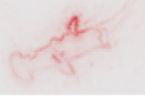

Image feature engineering#
Earlier approaches to image processing relied heavily on feature engineering by hand
Using edges to identify shape: edges are sharp changes in color
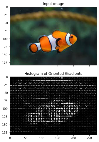
Some popular image features developed at these times
HOG (Histogram of Oriented Gradients) - Looking at changes in pixels
SIFT (Scale Invariant Feature Transform)
SURF (Speeded-Up Robust Feature)
The ideal feature information#
As an ideal, we want the model itself to find the best features to fulfill its task
How can a model map the high-dimensional image space to a lower dimensional subspace?
In which each image is represented by a long feature vector that behaves like structural data
In the following we try to find a model that can achieve this
Linear models for image modeling#
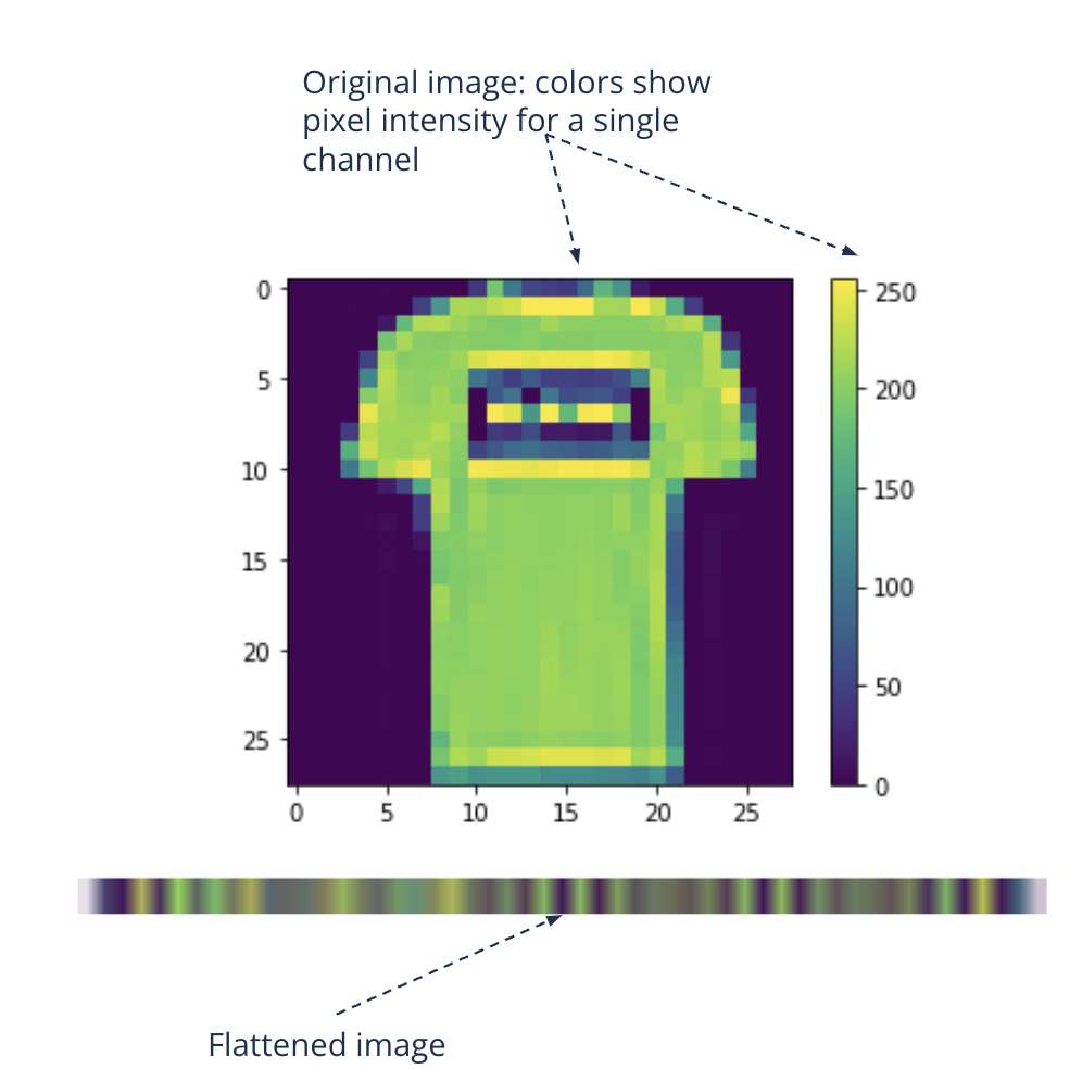
How to prepare the image data for a linear model?#
Given an image with height and width:
We could flatten the 2-dimensional tensor into a 1-dimensional one
Then just concatenating the channels therein
Given the label to be one of [T-shirt, Trouser, Pullover, Dress, Coat, Sandal, Shirt, Sneaker, Bag, Ankle boot]:
The label is represented by an integer between 0 and 9
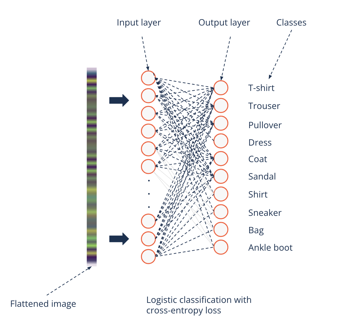
Logistic regression#
The logistic classification works on image data
On the MNIST Fashion dataset it reaches a 86% accuracy
That is almost a 15% error that could become costly in business
Can we improve modeling these image data?
Drawbacks of linear models#
Remember the TensorFlow playground
Linear models perform bad on non-linear data
Complex structures in data are hard to capture for linear boundaries
We need models capable of complex relationships between pixels
They must be able to approximate non-linear functions of high complexity
Such models must be able to do the feature engineering themselves
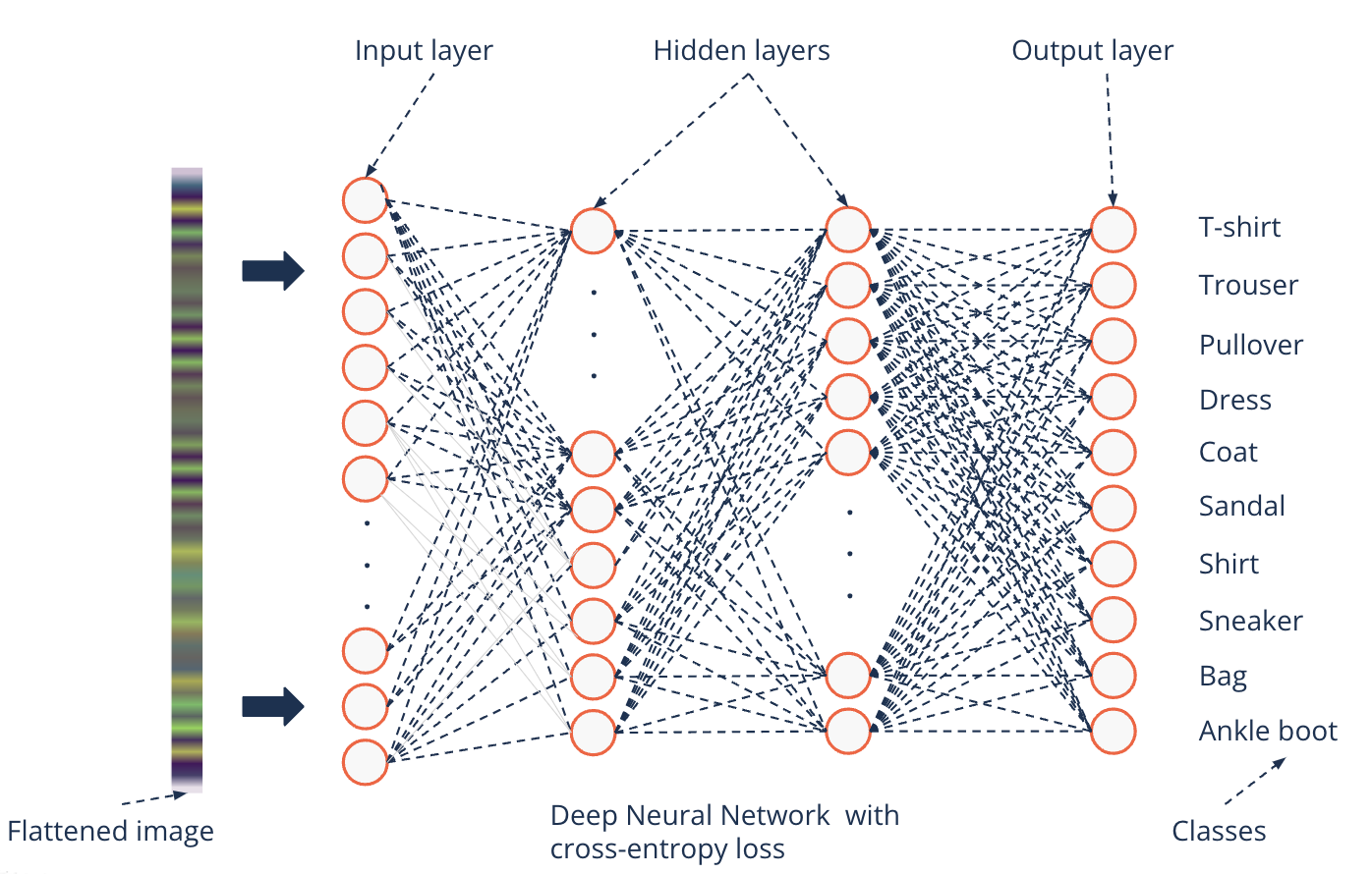
Deep Neural Networks for image modeling#
Deep Neural Networks perform better on image data#
Remember
Non-linear activation functions enable networks to model nonlinear functions
Hierarchy of neurons through layers make a complex feature extraction possible
Deep Neural Network on MNIST Fashion gets to a 91% accuracy
Drawbacks of Deep Neural Networks in image modeling#
Theoretically we can build a very deep network and approximate any function to classify images (universal approximation theorem), but
Very deep networks have high risk of overfitting
Real-world images have way more pixels
DNNs are not transformation invariant but are not dependent on the order of pixels either
i.e. the relationship between pixels does not count
ImageNet Competition#
ImageNet is the largest image recognition competition
~1.2M images and 1,000 categories
Until 2011 feature engineering defined a dominant part for winning teams
Xerox XRCE team won by using Fisher Vectors (multi-dimensional SWIFT) and SVMs
2012 AlexNet improved significantly and presented an implicit feature extraction
The authors used a {convolutional neural network (CNN)}
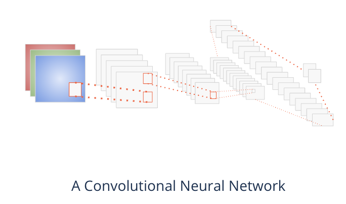
Convolutional layers#
Introduction#
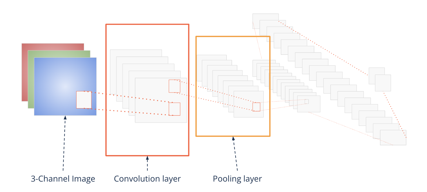
A convolutional neural network consists of two special layers:
Convolutional layers
Pooling layers
In the following we will consider these layers in detail
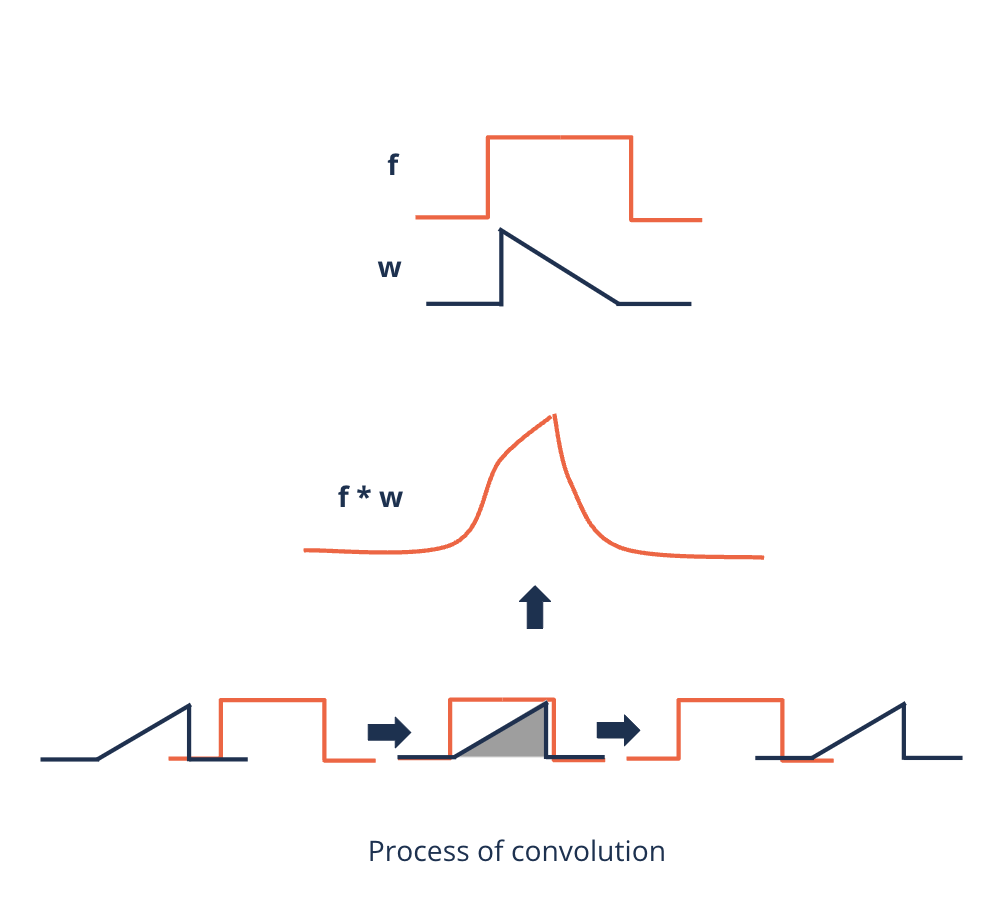
Convolution as a grouping of information#
We found out that the local relationships between pixels in an image contain important information
How can this relationship be captured?
Convolutional layers use a special mathematical method to capture these relationships: a {convolution}
Intuitively, they take snapshots from all regions of an image and apply filters to them
How does a convolution layer work?#
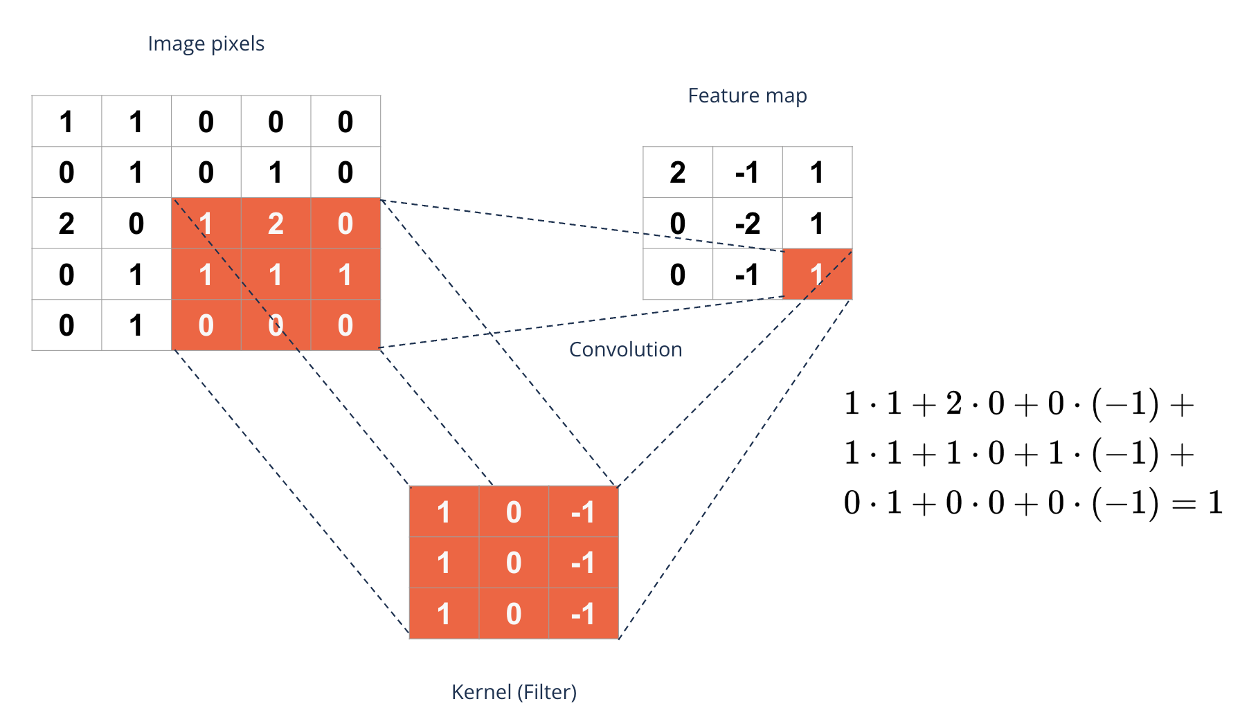
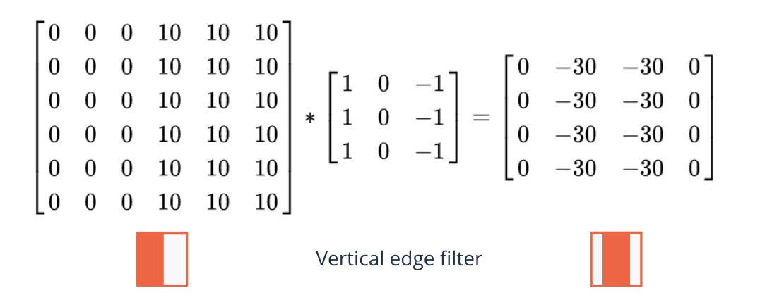
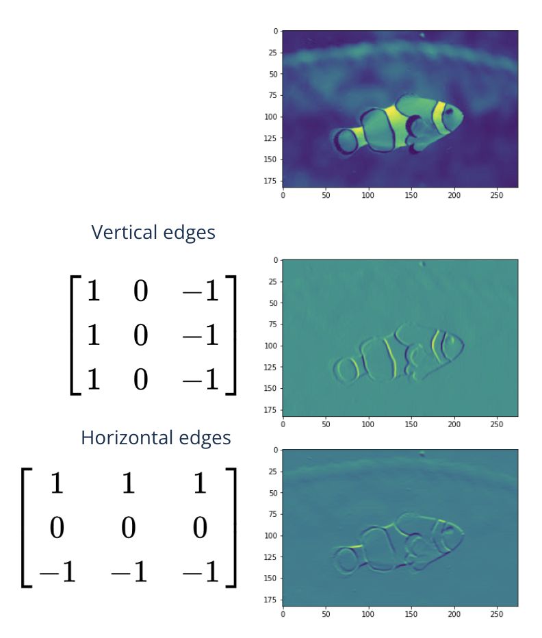
Edge detection#
A filter can detect different features in an image
Edges
Sharpening (edge detection + original image)
Blurring
Here we only look at edge detection to get an intuition how filtering works
Major idea of a convolutional layer#
Filters can be constructed by hand
Why not learning filter values {parameters} in training?
A convolutional layer contains many filters
Each filter forms during training
Each filter is of the same size and can process groups of nearby pixels
It looks at relationships between pixels {locality}
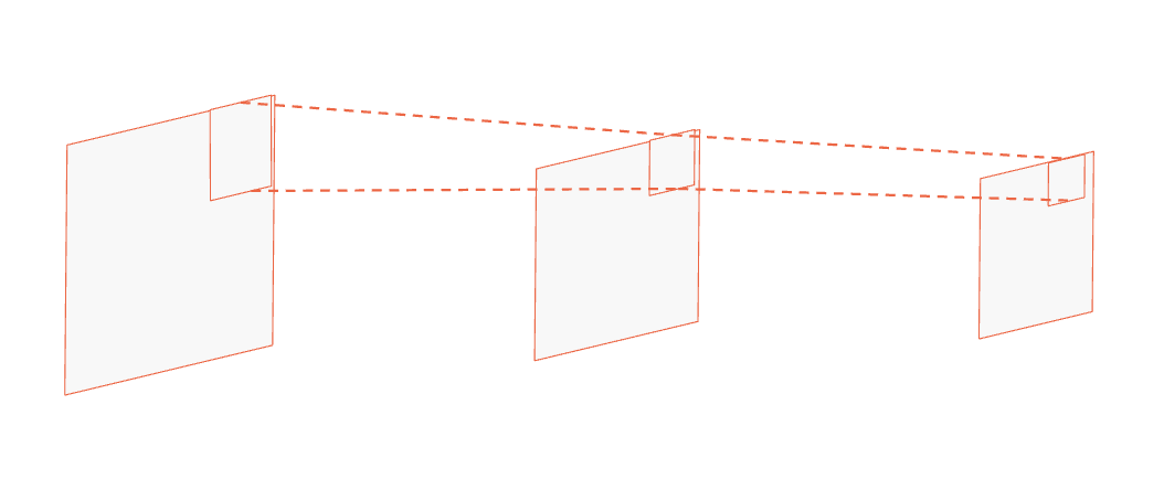
Reduction of dimensions#
Convolutional layers reduce the dimension of the image
A 28 x 28 picture filtered by a 3 x 3 kernel shrinks to a dimension of 26 x 26
This limits the number of convolutional layers applied to an image
At each layer the image shrinks
Formula for the resulting image dimension:
How can we build deep convolutional networks?#
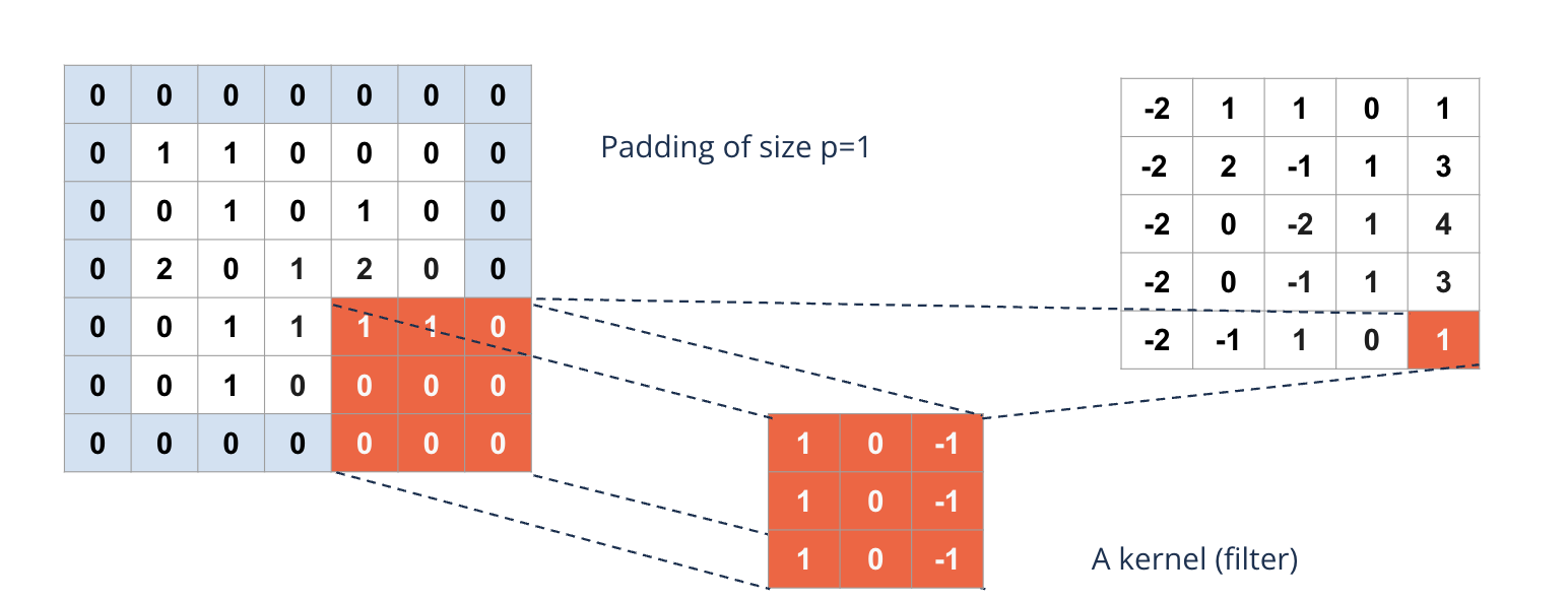
To avoid shrinking the image too quickly {padding} is applied
The image is ‘framed’ by zeros
A 28 x 28 image with a padding of 1 has dimension 30 x 30
WIth a kernel of 3 x 3 this results again in a 28 x 28 image
Formula for the resulting image size
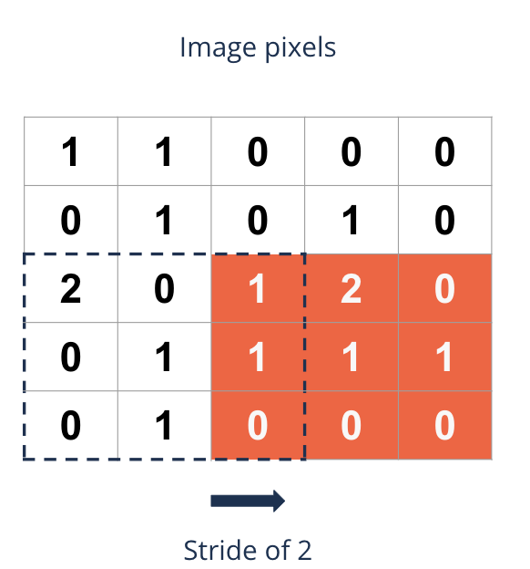
Making great strides#
Stride is the step size of the filter {kernel} by which it moves along the image
Sometimes a larger stride is desired
It reduces large image sizes to optimize memory usage and reduces computational costs
It reduces the risk of overfitting
Formula for the resulting image dimension (stride of 2):
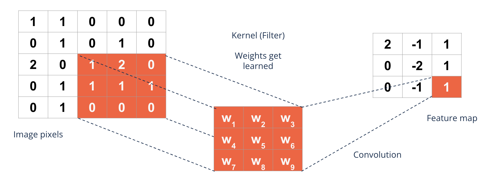
What happens during training?#
The filters {kernels} of a convolutional layer are variable
They get learned during training of the network
The network learns thereby optimal filters to fulfill its task
Stationarity principle#
There are features in an image that are essential and repeat themselves at different locations
Statistical signals are uniformly distributed:
These features have therefore also be detected at each location
This justifies {parameter sharing} which makes CNNs very parameter-efficient
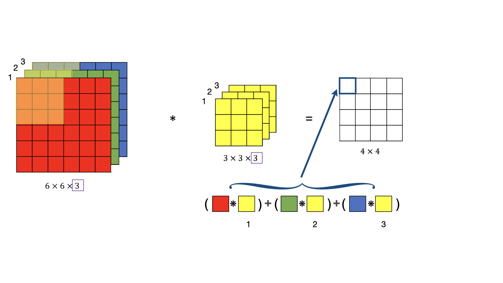
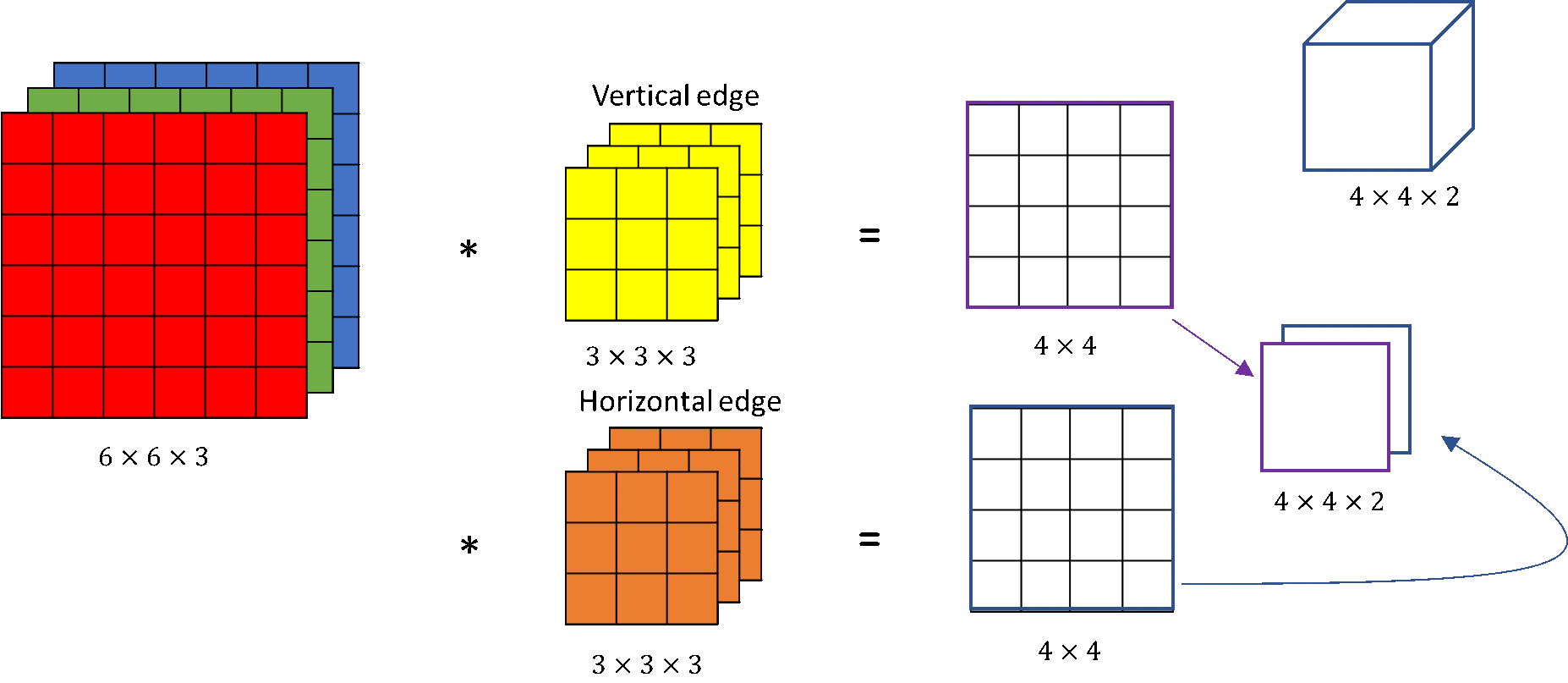
Working through the channels#
Color images have three channels
Convolutions take place across channels
I.e. a filter {kernel} is actually a cube
Working through the channels#
Color images have three channels
Convolutions take place across channels
I.e. a filter {kernel} is actually a cube
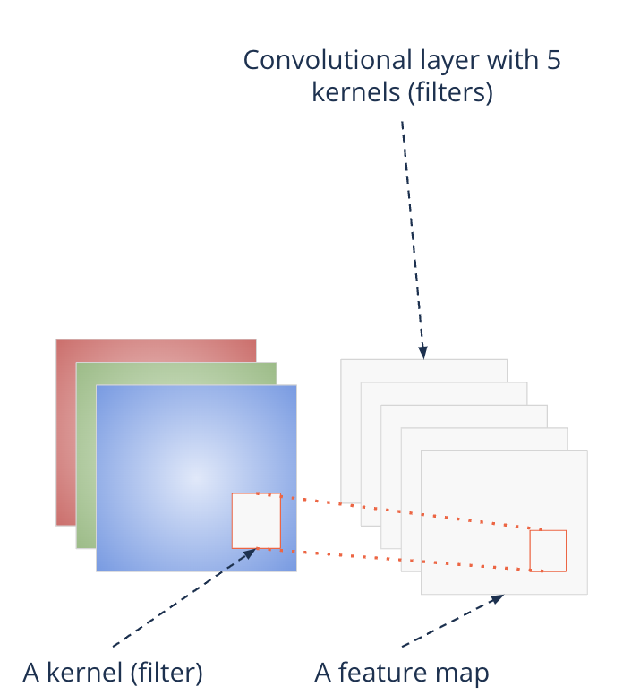
Per convolutional layer there are usually many filters applied
A filter per feature
I.e. the output is actually again multi-channel
The channel of the output is also called {feature map}
Parameter sharing is caring#
Remember the large image example (1280px x 720px):
27.6 Mio. parameters with 10 neurons in a DNN
110 MB in memory
Consider instead a convolutional layer with 64 filters of size 3x3 applied to a colour image
3x3x3x64 + 64= 1792 parameters!
7 KiB in memory
With parameter sharing we can train
faster
deeper networks
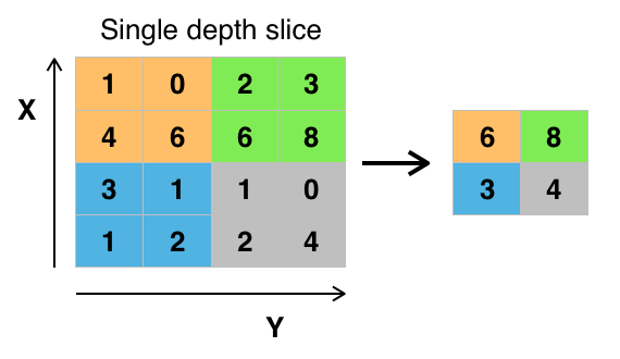
Pooling layers#
What is pooling?#
Pooling is aggregating features from {feature maps}
We pool over a certain window: we apply a summary of nearby pixels
The window is then moved across a feature map
Pooling reduces a feature map in size:
A 26 x 26 feature map with a 2x2 pooling layer reduces the feature map to dimension 25x25
Formula for the resulting dimension:
In practice pooling layers often use a stride corresponding to the kernel size: 2x2 kernel with stride of 2
How does a Pooling layer work?#
Why pooling?#
Pooling has two major effects:
It makes the network invariant to translations
Why pooling?#
Pooling has two major effects:
It makes the network invariant to translations
It strengthens the signal while it is running through the network
Compositionality principle#
Any image is compositional:
Features compose the image in a hierarchical manner
This justifies the use of multiple layers
Each layer composes features of the prior layer to a more complex one
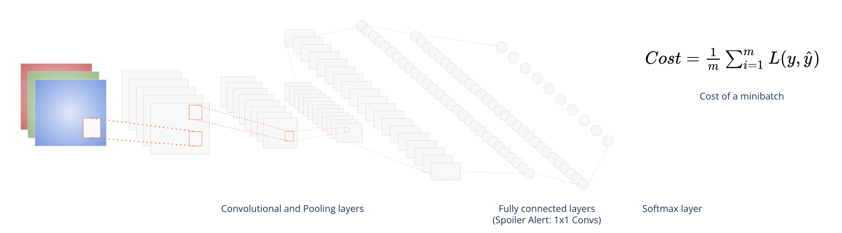
Building the network#
Stack layers together with a softmax or sigmoid layer at the end
Train with gradient descent to optimize parameters
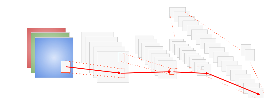
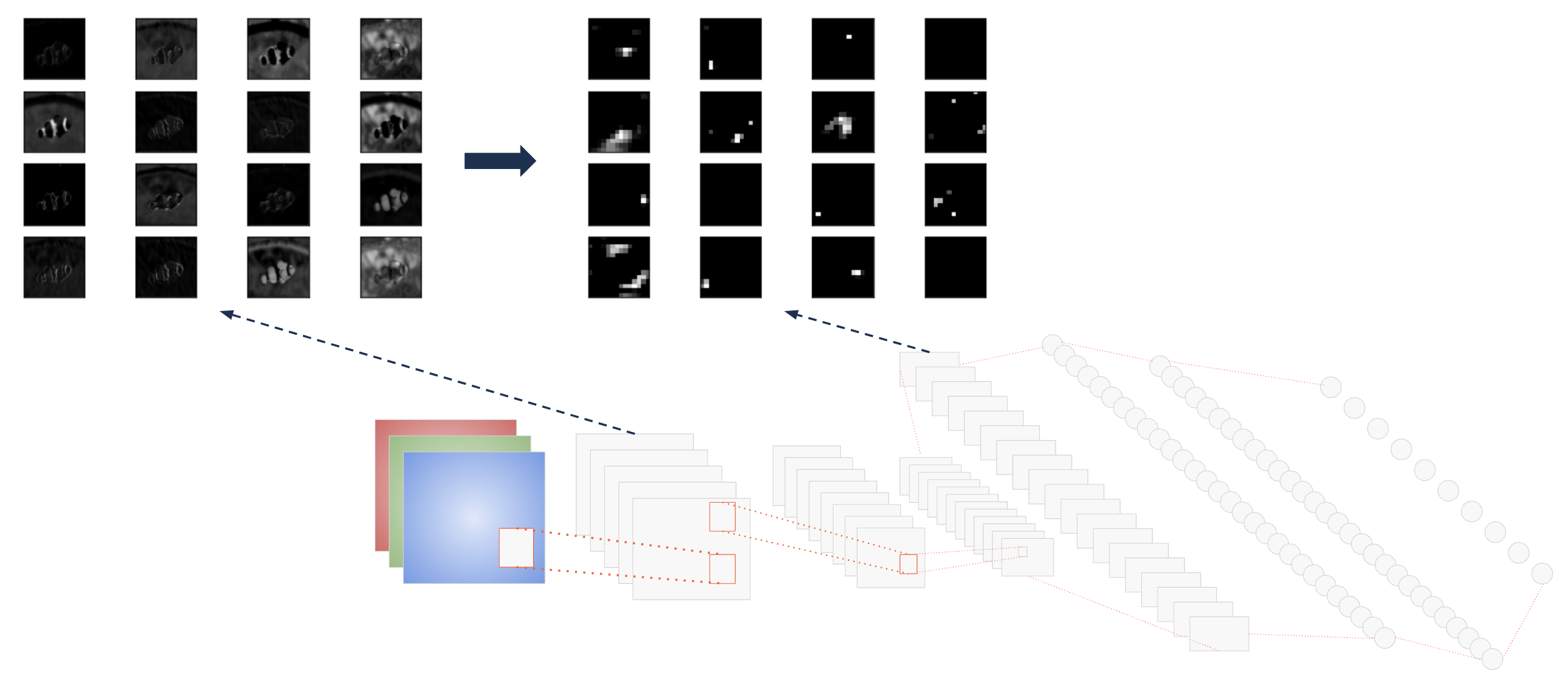
Feature extraction#
Hierarchical feature extraction
One pixel in deeper layer is connected to many pixels in shallow layer {sparse interactions}
Feature complexity grows in each layer
First layers learn simple structures, like edges and corners
Later layers learn complex structures like eyes, nose, etc.
Feature Extraction#
Data augmentation and transfer learning#
Challenges with convolutional neural networks#
Deep convolutional neural networks are data hungry
Imagine all the features it has to learn from images
Data sparsity then is a challenge
Could be too less, low-quality, too few variations
Two ideas have emerged in the deep learning community to overcome these problems:
Data augmentation
Transfer learning
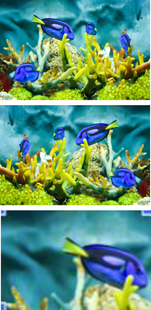
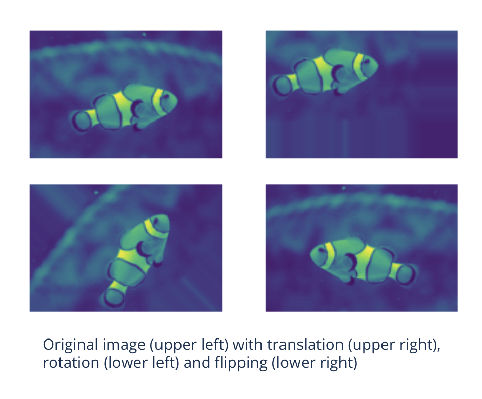
Data augmentation#
Idea:
Randomly transform images during training
Translate
Rotate
Zoom
Flip
…
Enlarges the data set by a significant factor
Makes the network more robust
Transfer learning#
Human beings learn tasks by transferring knowledge from other tasks they learned before
Can ANNs do the same?
They can - given some conditions
Same input distribution for both tasks
Well-learned representations on the first task
How does transfer learning work?#
A model is trained on many data for one task
For example classifying fishes
Then the upper layers are replaced by a classifier for the second task
For example classifying hymenoptera (wasps, bees, etc.)
This classifier for the second task gets trained
Usually significantly less data is needed for this task
Where do we get pre-trained models?#
Famous ML frameworks offer pre-trained models
GitHub:
Conclusion#
Image Modeling#
Image data is unstructured and shows regularly transformations
Locality, stationarity, compositionality principle
Image models are able to offer translation invariance
Special layers in image models are:
Convolutional layers: Extract features by filters
Pooling layers: Strengthen filter signals and make the net translation invariant
Data augmentation helps to increase the data size and robustness of the net
Transfer learning enables to use pre-trained models from one task for a second one
Resources#
Géron, A. (2019), Chapter 14: Deep Computer Vision Using Convolutional Neural Networks
Li, F.-F. and Johnson, J. (2017), Convolutional Neural Networks for Visual Recognition (much broader, lectures 1-5)
Image Feature Engineering:
Dalal, N. and Triggs, B. (2005), “Histograms of Oriented Gradients for Human Detection”, CVPR 2005. IEEE Computer Society Conference on. IEEE, 2005. S. 886–893
Lowe, D. (1999), “Object Recognition from Local Scale-Invariant Features”, ICCV ‘99 Proceedings of the International Conference on Computer Vision. Band 2, Seiten 1150–1157.
Lowe, D. (2004), “Distinctive Image Features from Scale-Invariant Keypoints”, International Journal of Computer Vision. Band 60, Nr. 2, Seiten 91–110, 2004
Bay, H. et al. (2006), “SURF: Speeded Up Robust Features”, European Conference for Computer Vision 2006
Drawbacks of deep neural networks:
Hornik (1991), “Approximation Capabilities of Multilayer Feedforward Networks”
Csáji (2001), “Approximation with Artificial Neural Networks”
ImageNet Competition:
Perronin and Sanchez (2011), “Compressed Fisher Vectors for LSVRC”
Krizhevsky et al. (2012), “ImageNet Classification with Deep Convolutional Neural Networks”
Strive:
Springenberg et al. (2015), “Striving for Simplicity: The All Convolutional Net”
Kong and Lucey (2017), “Take it in your stride: Do we need striding in CNNs?”
Data Augmentation:
LeCun et al. (1998), “Gradient-Based Learning Applied to Document Recognition”
Krizhevsky et al. (2012), “ImageNet Classification with Deep Convolutional Neural Networks”
Wang, J. and Perez, L. (2017), “The Effectiveness of Data Augmentation in Image Classification Using Deep Learning”
Transfer Learning:
Caruana, R. (1995), “Learning Many Different Tasks at the Same Time with Backpropagation”
Yosinski, J. et al. (2014), “How transferable are features in deep neural networks?”
Weiss, K. et al. (2016), “A survey of transfer learning”
Feature Extraction:
Garcia, D. et al. (2018), “On the Behavior of Convolutional Nets for Feature Extraction”
Zeiler, M.D. and Fergus, R. (2014), “Visualizing and Understanding Convolutional Networks”
Yosinski, J. et al. (2015), “Understanding Neural Networks Through Deep Visualization”