Ensemble Methods - Part 2#
Recap CART - Classification and regression trees#
CART (Classification and Regression Tree)#
General:
Finding the optimal split of the data is NP-complete.
CART uses a greedy procedure to compute a locally minimal MLE (Maximum likelihood estimation).
The split function chooses best feature and best value to split on.
Cost functions:
Regression \(\rightarrow J(b)=\frac{1}{n}\sum_{i=1}^{n}{(y_{i}-\hat{y_{i}})^2}\) (MSE)
Classification \(\rightarrow I_{G}(p)= 1-\sum_{i=1}^{J}\,p_{i}^{2}\) (Gini impurity)
CART#
Regularisation:
pruning to avoid overfitting
Grow a full tree and then prune e.g.
max_leavesmax_depthmin_sample_size
CART - pros and cons#
| PROS | CONS |
|---|---|
| white box model - easy to interpret | not very accurate ... |
| can handle mixed data, discrete and continuous | greedy nature of constructing |
| insensitive to transformations of data... split points based on ranking | trees are unstable, small changes to the input can lead to large changes in tree structure |
| relative robust to outliers | tend to overfit (aka high variance estimators) |
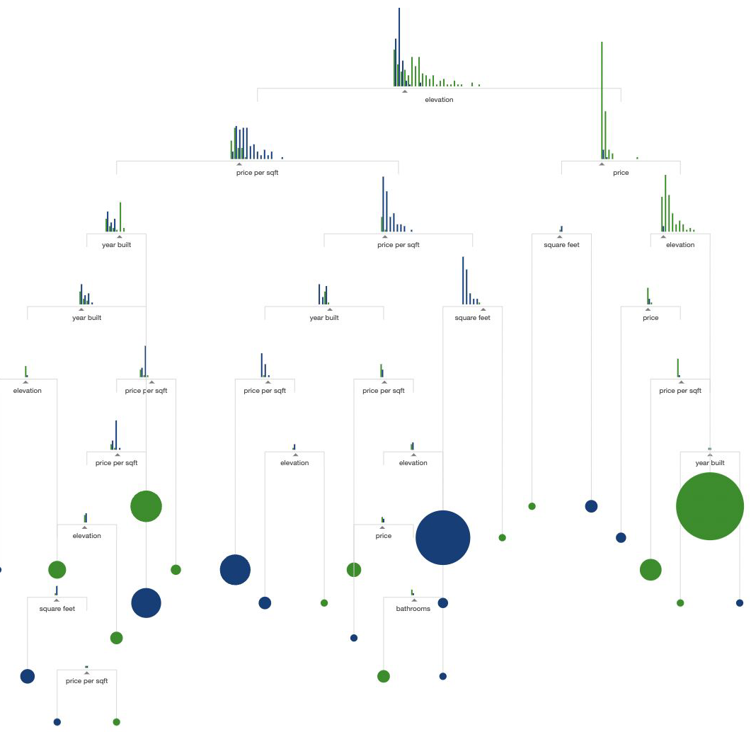
Trees being unstable#
Q: Should you trust and follow a single CART?
Changes in your trees can lead to different structure and maybe different decisions
As in investment, it is not advisable to lay all eggs in one basket
Trees being greedy and overfitting#
How to find out what to order at the restaurant?
Try everything!
… and then order what you liked best.Ask your friends to try something,
find out which they preferred more and try those maybe?
Q: Which do you find more feasible?


Wisdom of Crowds Theory#
Diversity of opinions
Independence of opinions
Decentralisation
Aggregation
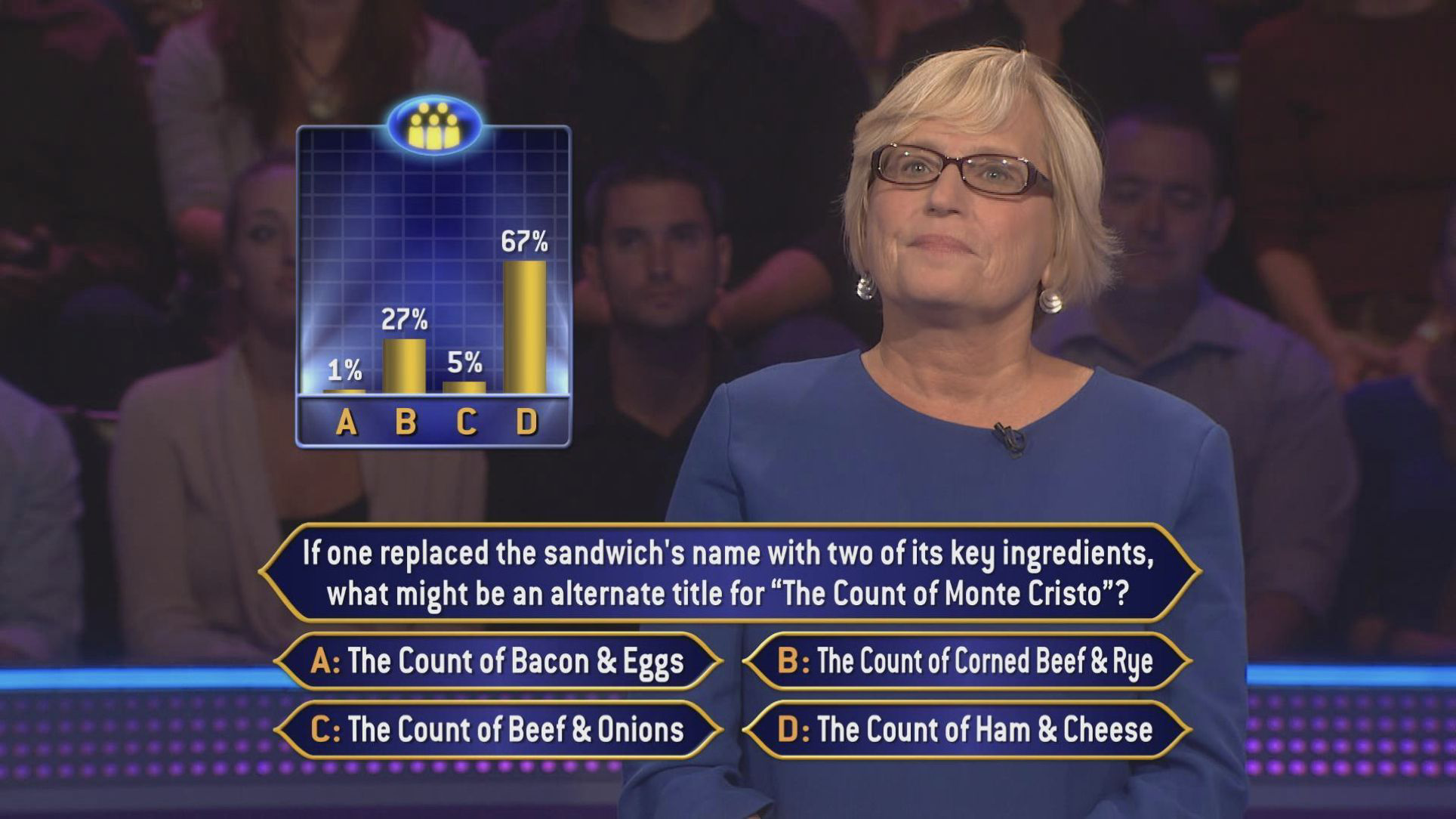
Who Wants to Be a Millionaire 💸 // 📖 Wikipedia#
| Who Wants to Be a Millionaire 💸 | Wikipedia 📖 |
|---|---|
| Each person has private information. | |
| The audience members should have opinions of their own. | Wikipedians have opinions of their own. |
| Independence of opinions. | |
| There might be some small local effects. | Wikipedians often don’t know each other. |
| Decentralisation | |
| Trivia knowledge isn’t specialised. People can make educated guesses. | Wikipedia is decentralized by definition. Single-author pages require review. |
| Aggregation | |
| People chose the most popular vote: max() | Talk pages to discuss and mediate disagreements. Decisions by consensus or executive decision. Loss of independence or lack of aggregation. |
Reducing variance by aggregation#

Ensemble learning… asking for more opinions and making a judgment call#
A collection of models working together on same dataset
Mechanism:
majority voting
There are different ways to do it:
bagging (same model on different parts of the data)
boosting (seq. adjusts for importance of observations)
stacking / blending (training in parallel and combining)
Advantages:
less sensitive to overfitting
better model performance

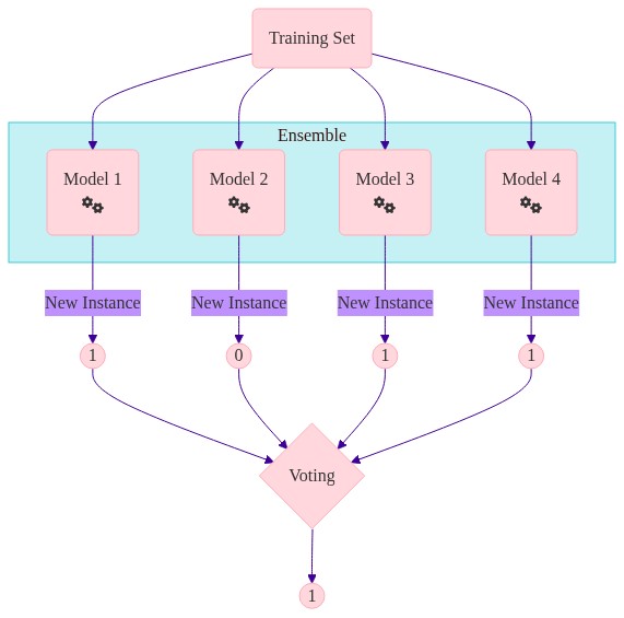
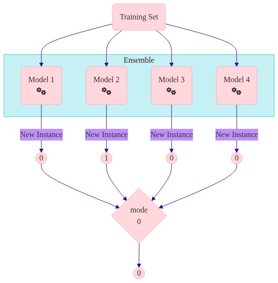
Majority Voting - how it works#
For each observation you have different predictions from different models
You need one prediction… so you aggregate
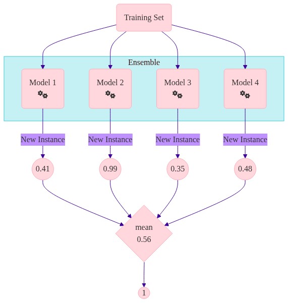
Aggregating the different models can be done in many ways e.g. averages, mode, median
Methods based on the values of the probabilities need to return calibrated probabilities.
Majority Voting - how it works#
For each observation you have different predictions. How do you aggregate this to get one value?
Soft voting tends to outperform hard voting.
Majority Voting - why it works#
Intuition: at observation level not all classifiers will be wrong in the same way at the same time
Prerequisites for this to work:
models need to be better than random, i.e. weak learners
you want the models to be different and that get translated in statistics to non-correlated or sufficiently independent or .. diverse
you need a sufficient amount of weak learners

A weak learner model has an average true positive rate slightly better than 50% and an average false positive rate slightly less than 50%.
Majority Voting - why it works#
What does it mean that the models are independent/ different?
If two weak learners would be correlated then a observation is likely to have same prediction by both weak learners.
Why do you think it is important?
Probability of an observation x to be misclassified by the ensemble learner is basically equivalent to it being misclassified by a majority of the weak learners.
 A weak learner is 51% right and 49% wrong
This can be proven by math. Feel free :D to try.. or
run 1000 coin toss experiments and aggregate.
Majority Voting - why it works#
\(X_i\) are independent identically distributed:
\(\text{Var} (X_{i})=\sigma^{2}\)
\(\text{Var} (\bar{X})=\text{Var}\left(\frac{1}{n}\sum_{i=1}^{n}X_i\right) = \frac{\sigma^2}{n}\), according to the central limit theorem.
Drop the independence assumption \(X_i\) are correlated by \(\rho\):
\( \text{Var}(\bar{X})=\rho\sigma^{2}+(1-\rho)\frac{\sigma^{2}}{n}\)
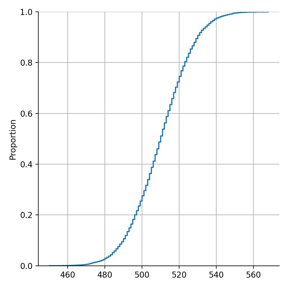
Example of weak learners#
Chances to be wrong with m = 1000 weak learners.
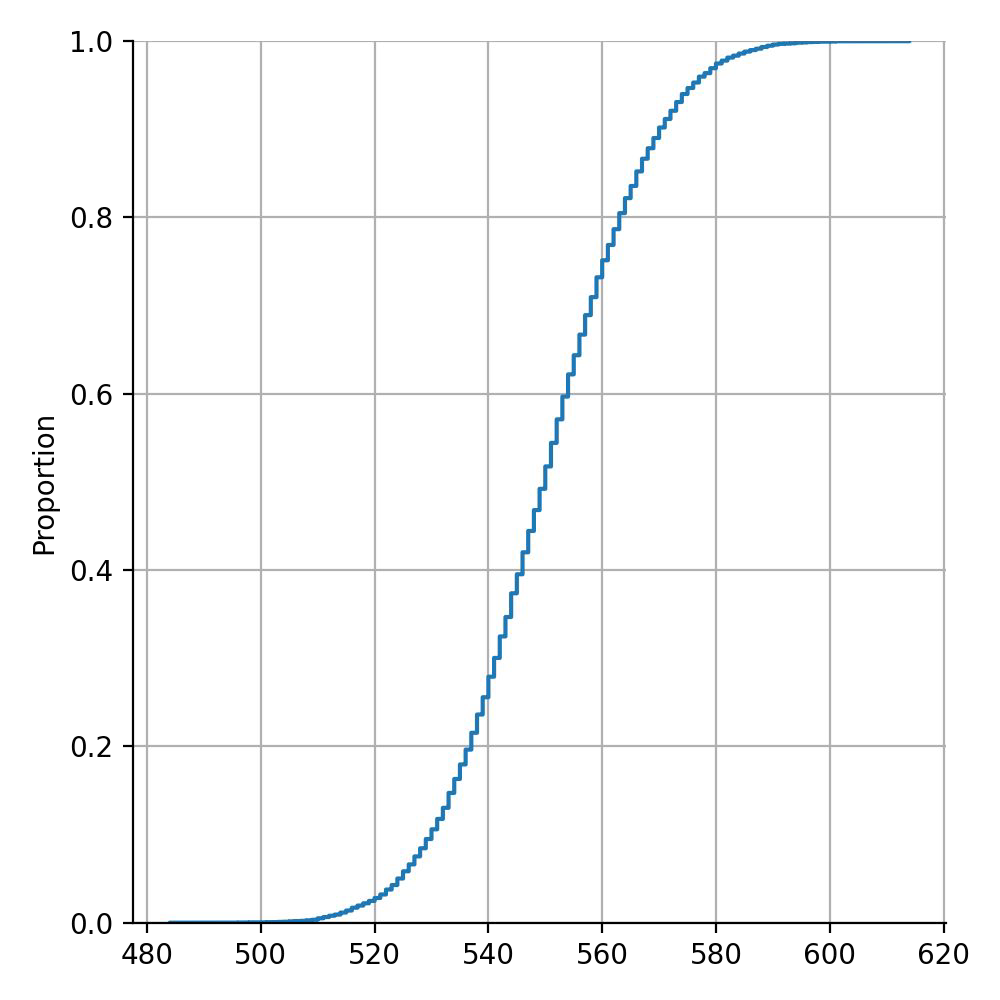
Example of weak learners#
Chances to be wrong with m = 1000 weak learners.
How does my model look as an ensemble model?#
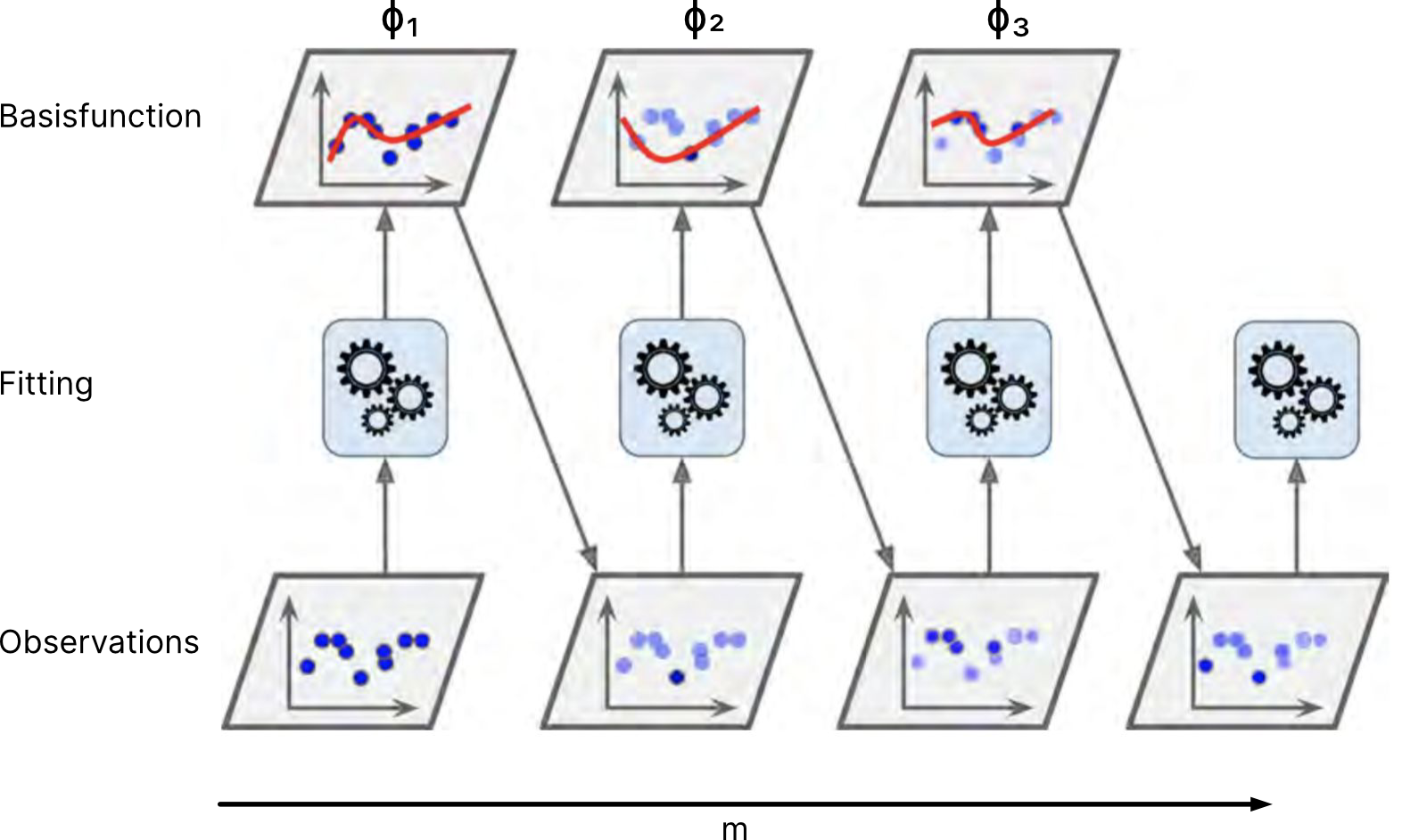
Adaptive basis function models#
This framework covers many models: decision trees, neural networks, random forest, boosting trees and so on… basically we have m parametric basis functions.
How does the formula look like for a decision tree?
How do I produce different models with the same data?#
I. Bagging#
Bagging#
Bootsprap aggregating
Training \(m\) different trees on different subsets of data chosen randomly with replacement.
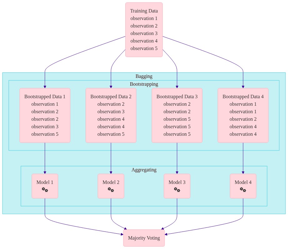
Running same learning algorithms on different subsets can result in still highly correlated predictors.
Random forest#
Random forest is a technique that tries to decorrelate the predictors
randomly chosen subset of input variables (features)
leading to different features used at each node
randomly chosen subset of data cases (observations)
leading to out of bag instances
Random forest gain in performance but lose in interpretability.
Grow a forest rather than a tree#
Ensemble of decision trees
Trained using bagging for selecting the train data
Uses a random subset of features at each node
Out-of-Bag Evaluation#
For each model, there are instances that are not trained on (because of the replacement). They are called out-of-bag instances (oob).
oobs are ideal for evaluation even without a separate validation set (out of bag error)
Random patches and Subspaces#
Why not sample the features too?
Random patches: sampling both features and instances
Random subspaces: Sample features only
Can be used for getting feature importance (How ?)
Extra-Trees - Extremely Randomized Trees#
Changing how we build the trees to introduce more variation
all the data in train is used to build each split
to get the root node or any node: searching in a subset of random features, the split is chosen randomly
random selection → Saves a lot of computational power
Accuracy vs variance#
Accuracy
Random Forest and Extra Trees outperform Decision Trees
Variance
Decision trees → high
Random Forest → medium
Extra Trees → low
II. Different models#
Using different models#
Really different models, not necessarily weak models. So you could use 3 or more of different types:
decision trees
random forest
neural networks
SVMs
NBs
KNN
Ridge Classifier
…
IV. Boosting#
Boosting#
A greedy algorithm for fitting adaptive basis function
Where:
\(\phi_{m}\) are generated by a weak learner
the weak learner is applied sequentially to weighted versions of the data
more weight is given to examples misclassified by earlier rounds
the weak learner can be any regressor or classifier but it is common to use CART → decision tree

Boosting algorithm#
INIT
Every instances has the same weight
LOOP
(Weights of instances incorrectly predicted are increased.)
Model is trained
All models predict
The predictions are weighted by their accuracy and added
Boosting#
We do not go back and adjust earlier parameters → method is called forward stagewise additive modeling
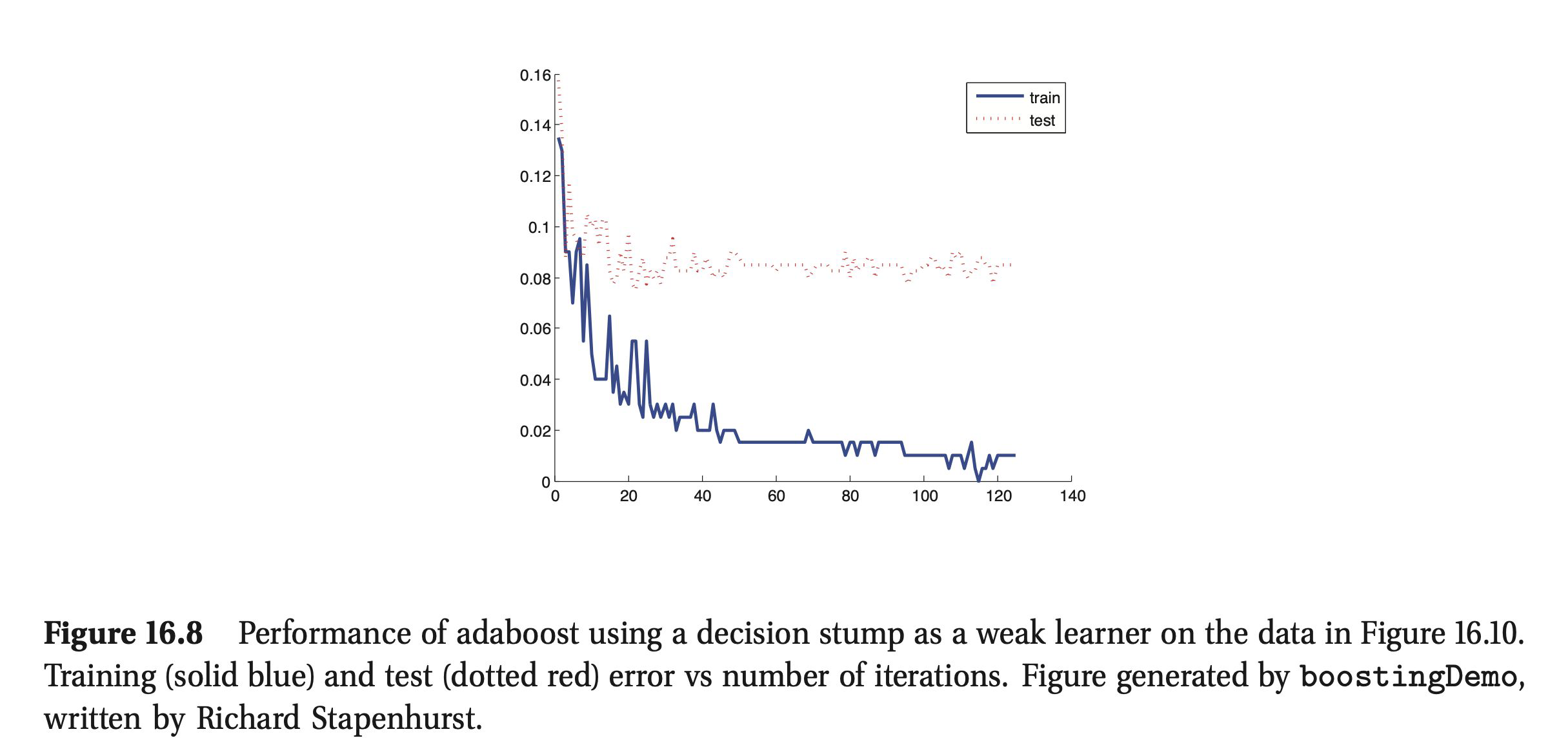
The problem of overfitting#
Boosting is very resistant to overfitting. Boosting can be interpreted as a form of gradient descent in the function space.
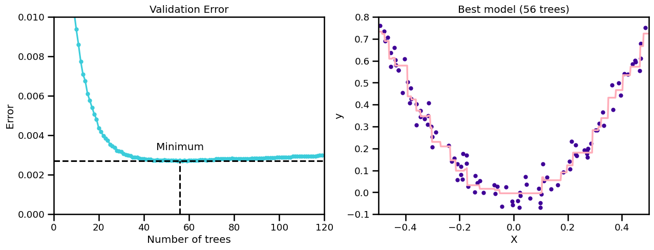
Early stopping#
How many models do we add?
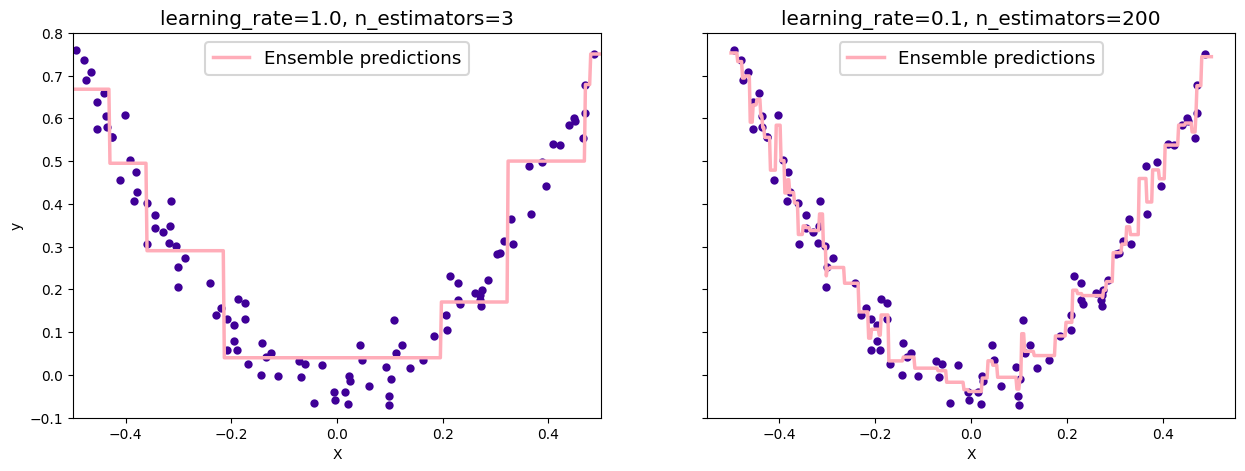
Early stopping#
How many models do we add?
Examples for boosting algorithms#
AdaBoost
LogitBoost
Gradient Boost
Stochastic Gradient Boost
XGBoost (eXtreme Gradient Boost)
Boosting optimization#
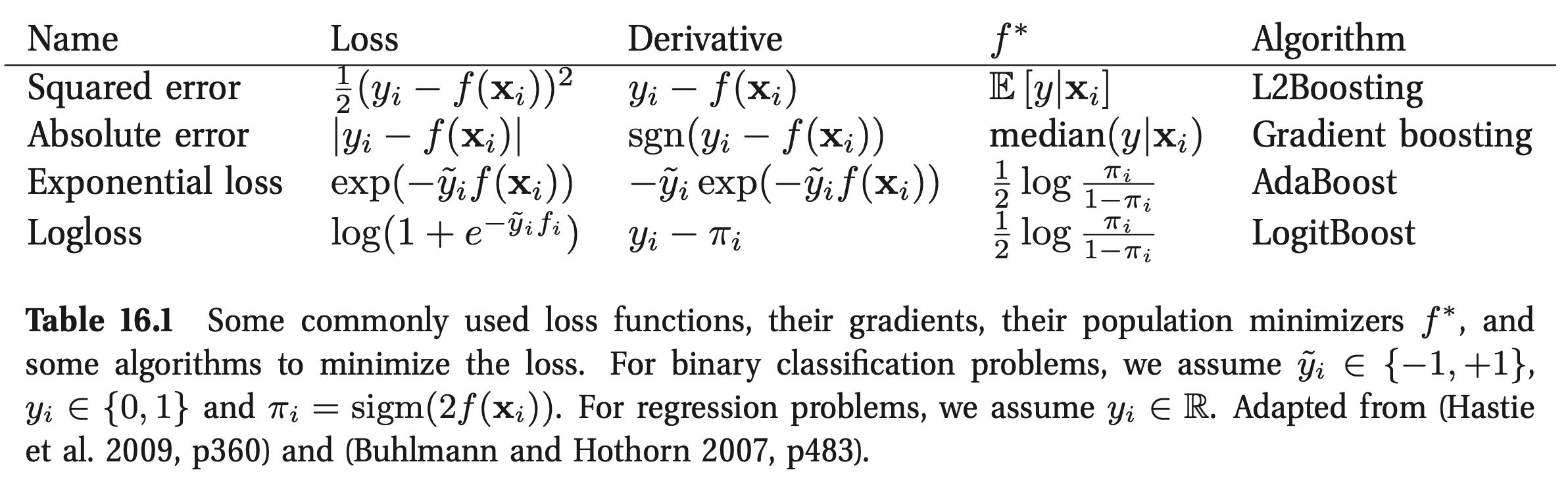
Boosting methods Adaboost#
loss function is exponential
it’s putting lots of weight on misclassified examples
after many iterations it can “carve out” a complex decision boundary
slow to overfit
sensitive to outliers
probability estimates from f(x) cannot be recovered
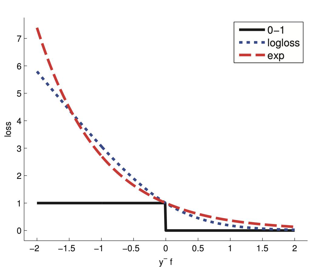
Boosting methods Logitboost#
loss function is logloss
punishes mistakes linearly
one can extract probabilities from f(x)
Boosting methods Gradient boosting#
sequentially adding predictors
based on the errors of the preceding model
instead of minimizing the loss function at each stage to get the parameter update for f, we get \(g_m\) the gradient for the loss of \(f_{m-1}\)
\(f_m=f_{m-1}- \rho_m g_m\) , where \(\rho\) is the step length chosen by minimising the error
Target outcomes for each case are set based on the gradient of the error with respect to the prediction.
Stochastic Gradient Boosting#
use a random subset of instances
higher bias but lower variance
speeds up training
XGboost - Extreme Gradient Boosting#
optimized implementation
scalable
automatic implementation of early stopping and many more
Chen, T. and Guestrin, C. (2016): “XGBoost: A Scalable Tree Boosting System”
IV. Stacking#
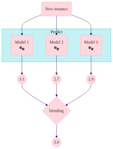
Use a model to aggregate#
train weak learners in parallel
combine by choosing the best for each observation
this will obviously overfit
using cross-validation to avoid overfitting
Applications: netflix competition winners in 2009
Blending (holdout) → Stacking (CV)
chart("""
flowchart TD
    A(New instance) --> B(Model 1
    fa:fa-cogs) --> F(( 3.1 )) --> J{blending
    } --> K((3.0))
    A --> C(Model 2
    fa:fa-cogs) --> G(( 2.7 )) --> J
    A --> D(Model 3
    fa:fa-cogs) --> H(( 2.9 )) --> J

    subgraph "Predict"
        B
        C
        D
    end
""")
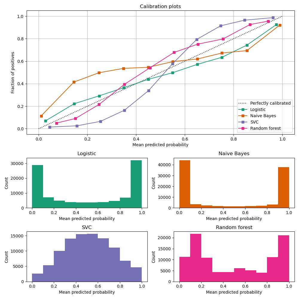
V. Classifier calibration#
Calibrated probabilities#
Fitting a regressor (called a calibrator) that maps the output of the classifier (decision_function or predict_proba) to a calibrated probability in [0, 1]
Interpretability#
Interpreting black box models#
Linear models are popular due to interpretability, but poor performance
Conclusions on the importance of a variable should be based on models with good accuracy
Some of the approaches for measuring the effect of variables:
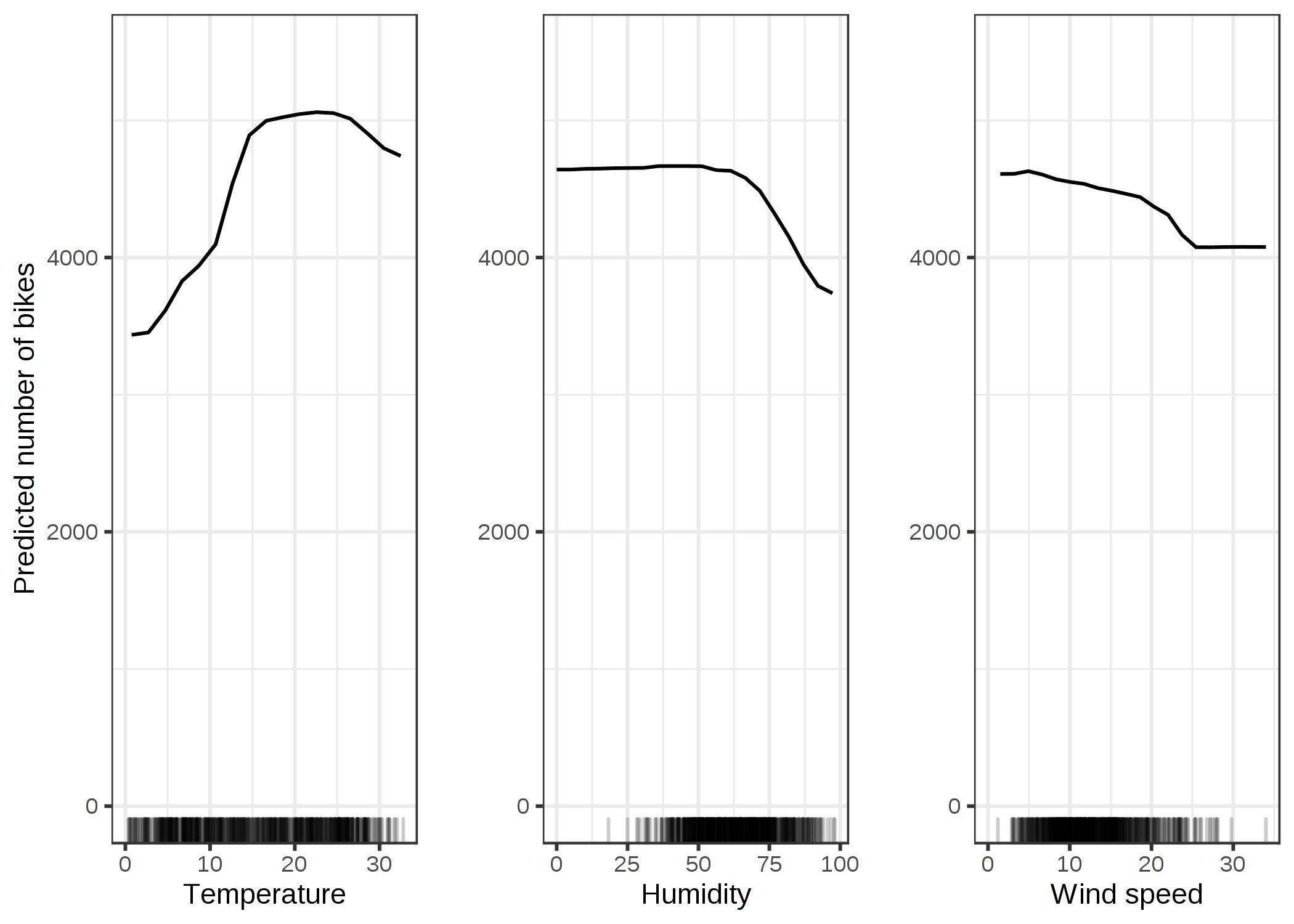
partial dependence plot
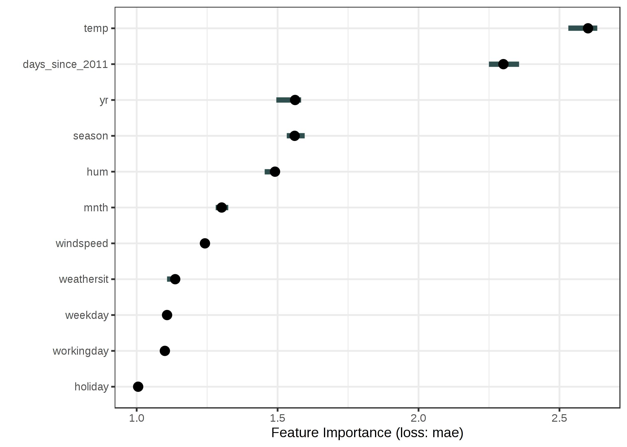
feature importance
shapley values
Partial dependence plots - PROS#
Intuitive: the partial dependence function at a particular feature value represents the average prediction if we force all data points to assume that value
causal interpretation (for the model)
Partial dependence plots - CONS#
maximum 2 features per plot
assumption of independence between features
some pd plots do not show the feature distribution
Permutation feature importance - PROS#
nice interpretation: the loss if the feature is removed
it takes into account the interaction with other features
does not require retraining the model
Permutation feature importance - CONS#
unclear if to use train or test data
linked to the error of model
need access to true outcome of model
doesn’t deal well with correlated features
References#
Machine learning a probabilistic perspective - Kevin p. Murphy