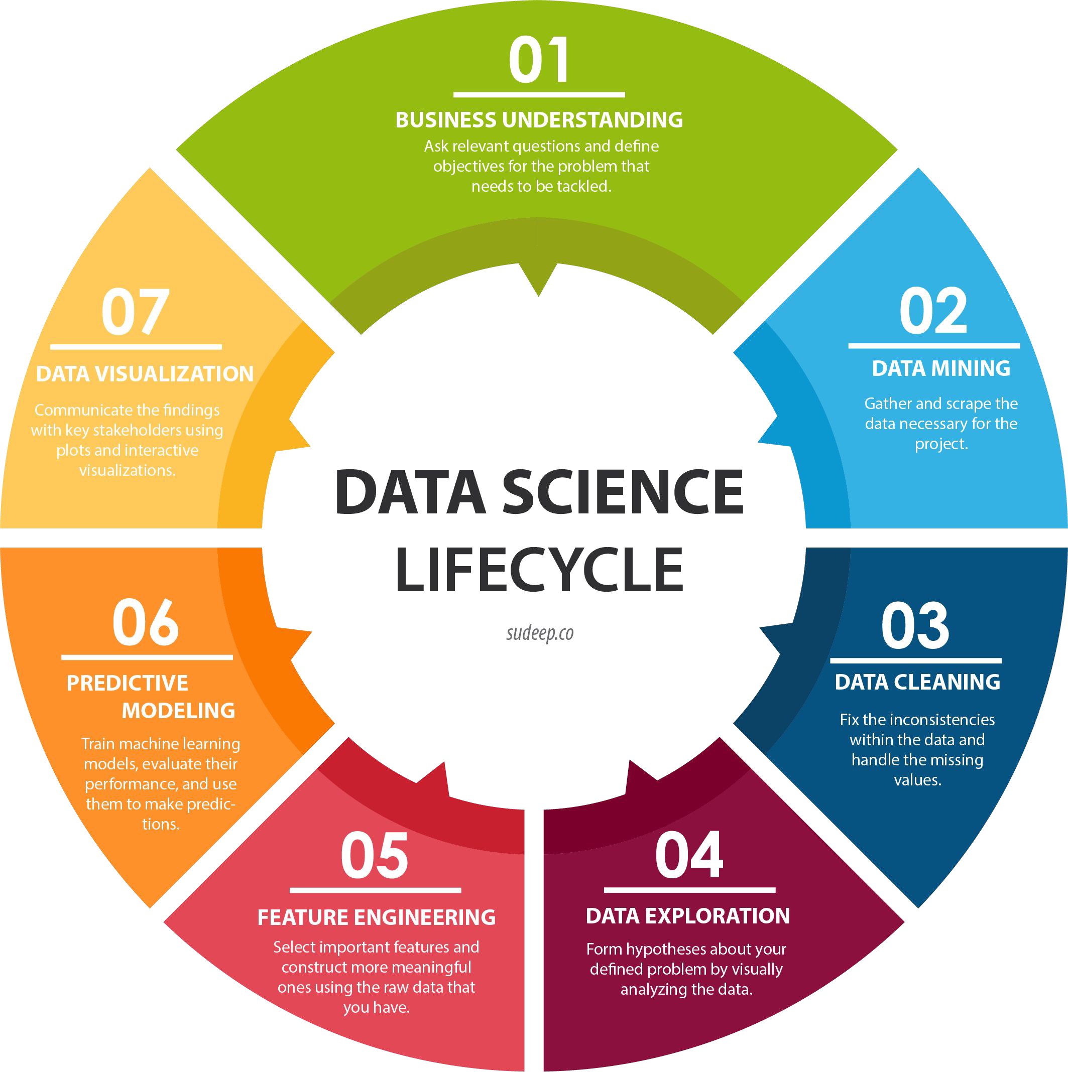
Orientation#
Where are we now?
06 PREDICTIVE MODELING:
select a ML algorithm
train the ML model
- evaluate the performance
make predictions
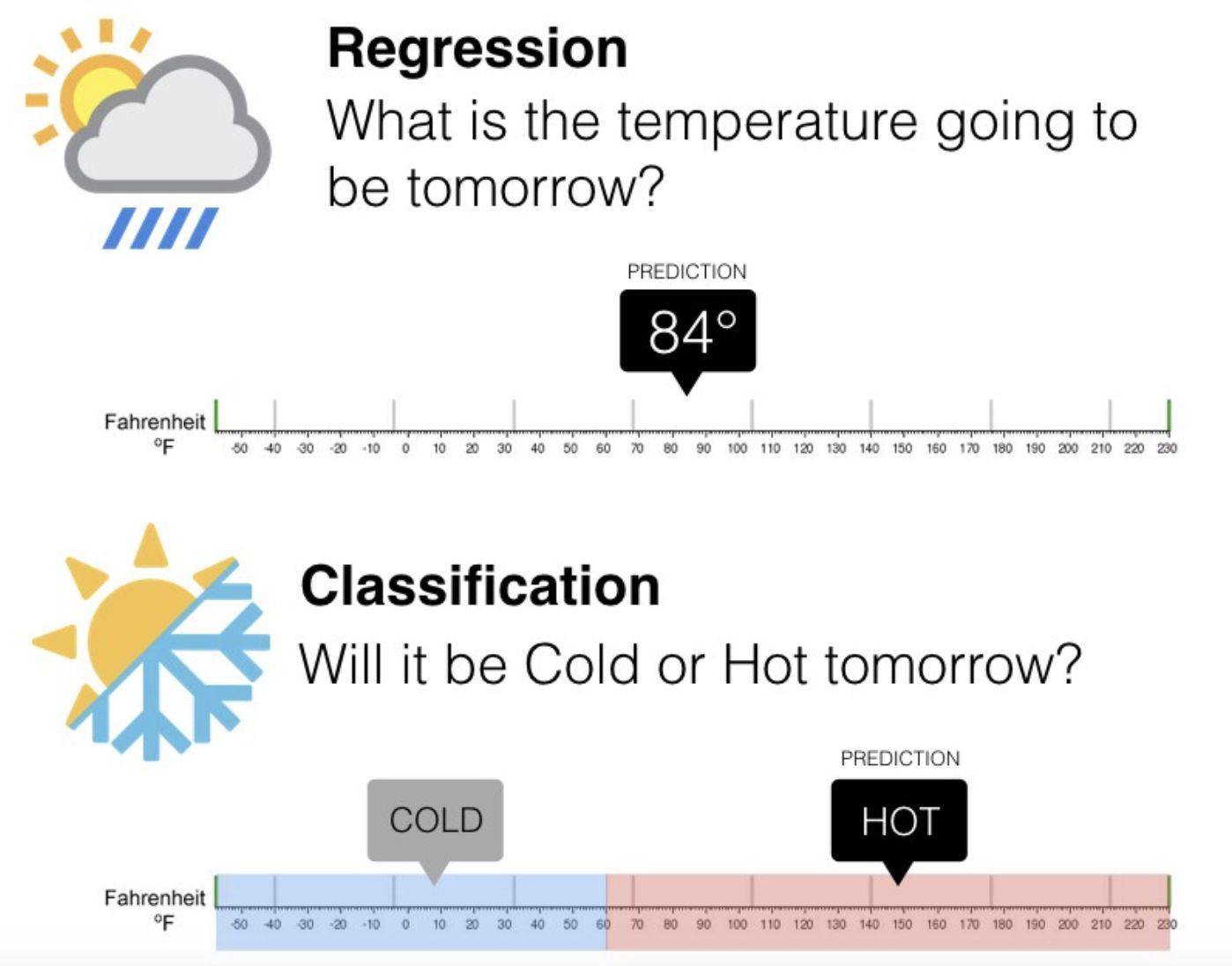
Evaluate model performance#
Regression Metrics (R-squared, RMSE…)
Classification Metrics (accuracy, precision, recall…)
Custom Metrics
→ e.g. based on the worst case scenarios of your product
Short recap on regression metrics#
What Metrics do we have to evaluate model performance?#
R2 (R-squared)
MSE (Mean Square Error)
RMSE (Root Mean Square Error)
MAPE (Mean Absolute Percentage Error)
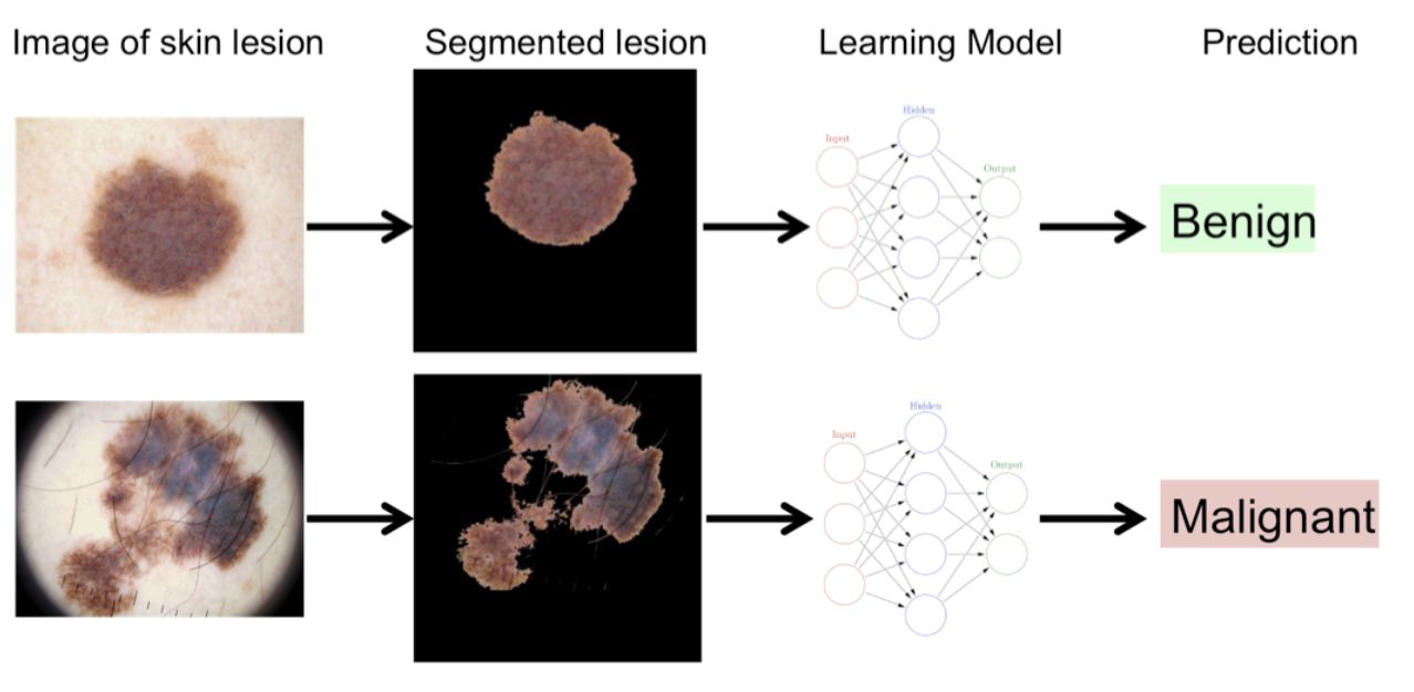
Let’s talk about classification#
Confusion Matrix#
Counts how often the model predicted correctly and how often it got confused.
False Positive: false alarm / type I error
False Negative: missed detection / type II error
| Predicted | |||
|---|---|---|---|
| Negatives | Positives | ||
| Actual | Negatives | TN | FP |
| Positives | FN | TP | |
Accuracy#
How often the model has been right.
| Predicted | |||
|---|---|---|---|
| Negatives | Positives | ||
| Actual | Negatives | TN | FP |
| Positives | FN | TP | |
Drawbacks#
When one class is very rare it leads to false conclusions
Here, Accuracy is 94 %
But 5 out of 6 positives have been predicted incorrectly
| Predicted | |||
|---|---|---|---|
| Negatives | Positives | ||
| Actual | Negatives | 93 | 1 |
| Positives | 5 | 1 | |
Accuracy might not be good enough#
Precision and Recall#
Focus on positive class
Number of True Negatives are not taken into account
When trying to detect a rare event
The number of negatives is very large
What proportion of actual positives was predicted correctly?#
The TPR is also called sensitivity or recall.
Here, the True Positive Rate is ⅙ (~16.67%).
| Predicted | |||
|---|---|---|---|
| Negatives | Positives | ||
| Actual | Negatives | 93 | 1 |
| Positives | 5 | 1 | |
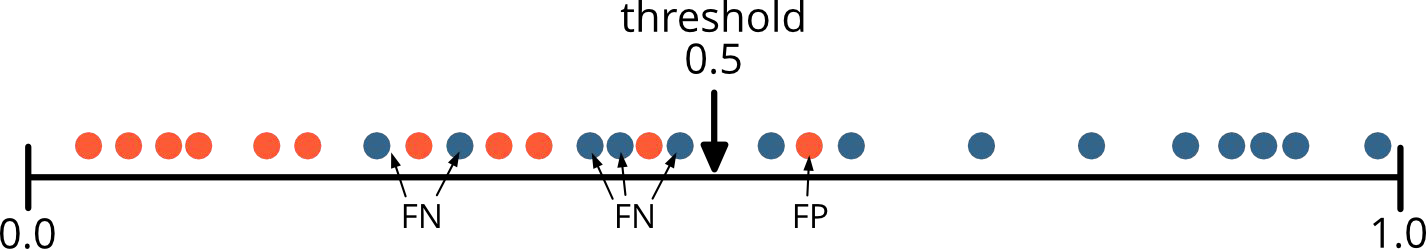
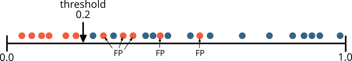
Tweaking the model#
Every model has a threshold that discerns positive from negative predictions.
Typically, instances will get predicted positive if the probability for that is \(\geq\) 0.5.
| Predicted | |||
|---|---|---|---|
| Negatives | Positives | ||
| Actual | Negatives | 93 | 1 |
| Positives | 5 | 1 | |
Tweaking the model#
The lower the threshold the more instances get predicted positive.
This will automatically raise the True Positive Rate (TPR) / Recall.
| Predicted | |||
|---|---|---|---|
| Negatives | Positives | ||
| Actual | Negatives | 93 | 1 |
| Positives | 5 | 1 | |
Now let’s tweak the model#
After tweaking the True Positive Rate (TPR) is at 100%.
But are we entirely happy?
| Predicted | |||
|---|---|---|---|
| Negatives | Positives | ||
| Actual | Negatives | 93 | 1 |
| Positives | 5 | 1 | |
| Predicted | |||
|---|---|---|---|
| Negatives | Positives | ||
| Actual | Negatives | 14 | 80 |
| Positives | 0 | 6 | |
What proportion of positive predictions are actually correct?#
Precision is 6/86 (~6.97 %), even lower as recall before tweaking!
But: if it’s too low or acceptable depends on the business case.
For detecting cancer it might be okay for the stakeholders.
→ Still, costs for screening millions of people might be very high.
| Predicted | |||
|---|---|---|---|
| Negatives | Positives | ||
| Actual | Negatives | 14 | 80 |
| Positives | 0 | 6 | |
Summary#
\(N_+ \) : the number of positives
\(N_- \) : the number of negatives
n = # observations
| Predicted | ||||
|---|---|---|---|---|
| Negatives / 0 | Positives / 1 | ∑ | ||
| Actual | Negatives / 0 | TN | FP | N- = FP + TN |
| Positives / 1 | FN | TP | N+ = TP + FN | |
| ∑ | N-hat- = FN + TN | N-hat+ = TP + FP | n = TP + FP + FN + TN | |
Precision-Recall Curve#
Plots Precision vs. Recall depending on the threshold.
If threshold is high:
→ Precision is close to 1.
→ Recall will be very low.
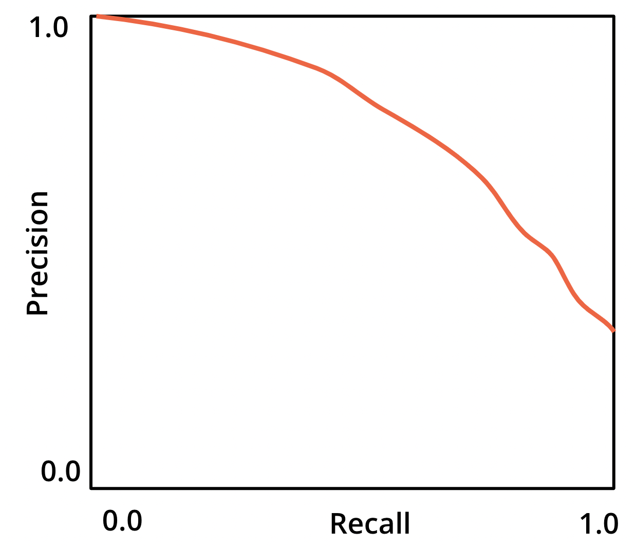
Precision-Recall Curve#
If threshold is effectively zero:
→ Predicting all instances as positives.
→ Recall will be 1.
→ Precision is equal to the share of positives.Goal: Get a threshold the stakeholder agrees on.
Starting point might be estimation of economic benefit and cost.
F1-Score#
Harmonic mean of precision and recall
Here the F1-Score is 13.08%
\(F_1 = 2\cdot\frac{Precision\;\cdot\;Recall}{Precision\;+\;Recall}\)
\(F_1 = 2\cdot\frac{7\cdot100}{7+100}=13.08\%\)
| Predicted | |||
|---|---|---|---|
| Negatives | Positives | ||
| Actual | Negatives | 14 | 80 |
| Positives | 0 | 6 | |
F1-Score#
The harmonic mean punishes low rates.
\(F_1 = 2\cdot\frac{Precision\;\cdot\;Recall}{Precision\;+\;Recall}\)
| Precision | Recall | F1-Score |
|---|---|---|
| 5% | 50% | 9% |
| 90% | 90% | 90% |
| 30% | 60% | 40% |
Let’s take negatives into the equation#
The amount of correct negative predictions is sometimes just as important
Spam vs. ham is just one example (email spam detection)

What proportion of actual negatives was predicted as positives?#
False Positive Rate
Here the FPR is: \(\frac{80}{80+14} = 85.11\%\)
| Predicted | |||
|---|---|---|---|
| Negatives | Positives | ||
| Actual | Negatives | 14 | 80 |
| Positives | 0 | 6 | |
What proportion of actual negatives was predicted correctly?#
True Negative Rate also called specificity
Here the TNR is: \(\frac{14}{80+14} = 14.89\%\)
FPR = 1 - specificity
| Predicted | |||
|---|---|---|---|
| Negatives | Positives | ||
| Actual | Negatives | 14 | 80 |
| Positives | 0 | 6 | |
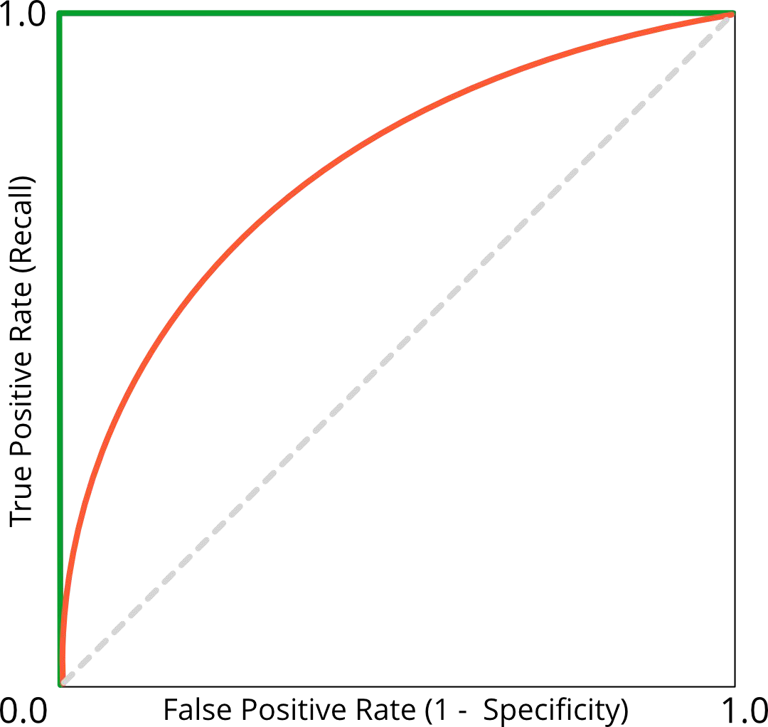
Receiver Operating Characteristic Curve (ROC Curve)#
TPR vs. FPR plotted for different thresholds
The 45° line is equivalent to throwing a coin
If all positives are correctly predicted and no negative is incorrectly predicted ROC curve would be the green curve
Aim: ROC curve as closely as possible to (0,1)
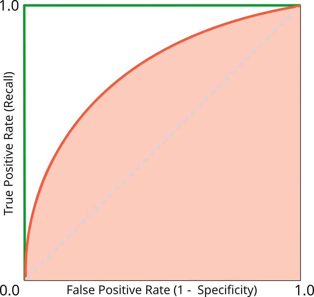
ROC and the Area Under the Curve (ROC AUC)#
Metric to compare different classifiers
Random classifier:
→ ROC AUC is 0.5
→ ROC curve is on the 45° linePerfect classifier:
→ ROC AUC is 1
Explanation of ROC curve#

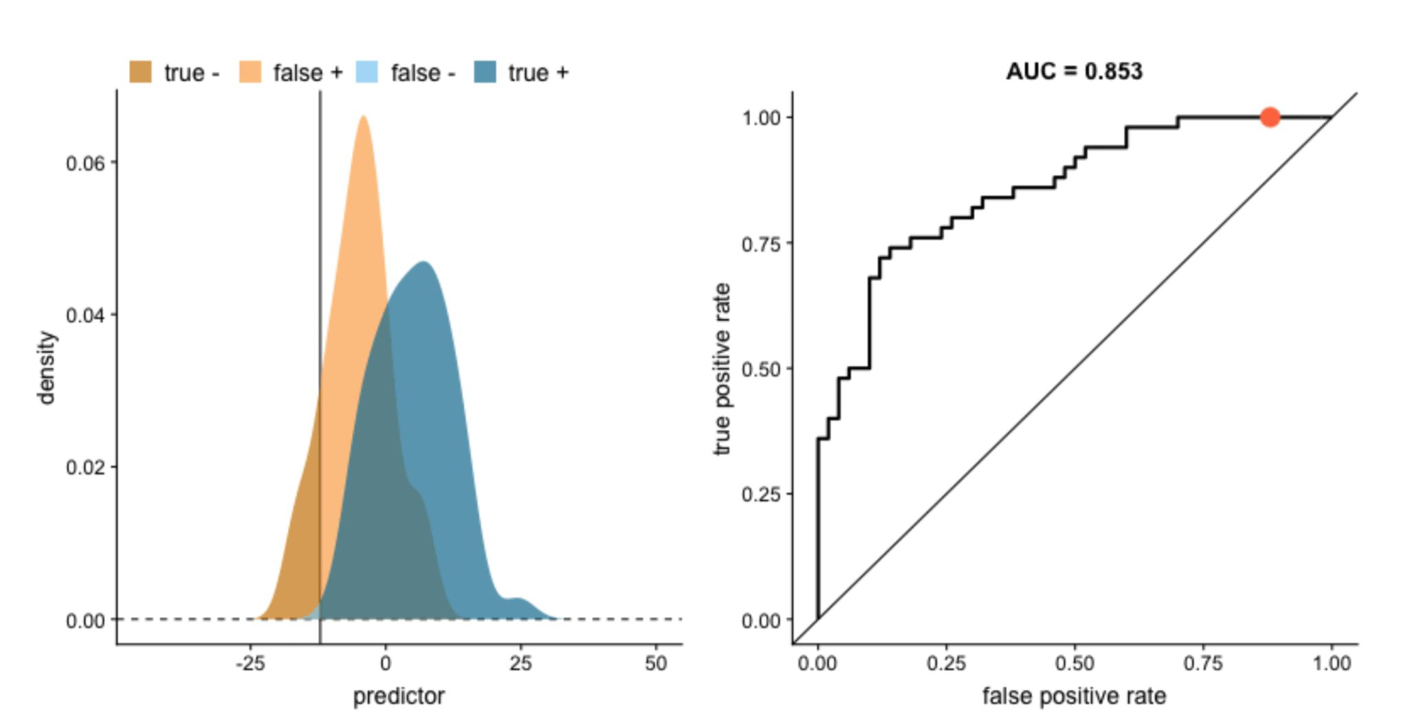
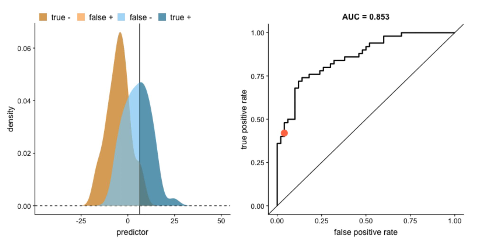
Explanation of ROC curve#

Imbalanced classes#

Going beyond aggregated metrics#
All the performance metrics we’ve seen today are aggregated metrics.
They help determine whether a model has learned well from a dataset or needs improvement.
Next step:
Examine the results and errors to understand why and how the model is failing or succeeding.
Why: validation and iteration
Validate your model → inspect how it is performing#
There are a lot of way to do this. You want to contrast data (target and/or features) and predictions.
Regression:
Looking at residuals, for example doing EDA on residuals and inspecting the outliers.
Classification:
One can start with a confusion matrix, breaking results in true class and predictions.
Resources#
roc-auc-precision-and-recall-visually-explained
Building Machine Learning Powered Applications - Emmanuel Ameisen