Artificial Neural Networks#
# If the graphviz pictures cause an error:
#(this was removed from requirements.txt file again, after it caused on github an error when running the jupyter book.)
#!pip install graphviz
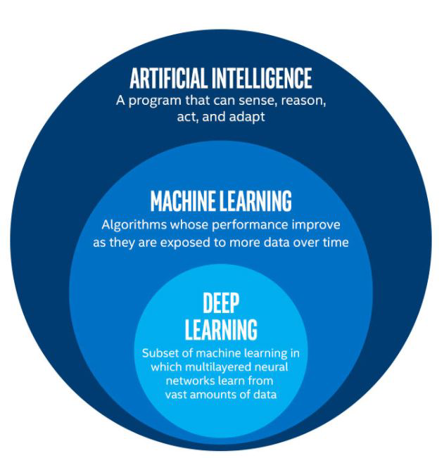
Adaptive basis function models#
remember ensemble models?
When and Why?#
non-linearity
many dimensions
…
When and why?#
Non linear hypotheses
Assuming this data: to this dataset you could apply logistic regression with a lot of nonlinear features including lots of polynomials
For 100 features, including the second order polynomials you get about 5000 features ~ \(O(n^2)\) features

When and why?#
Non linear hypotheses
Assuming this data: to this dataset you could apply logistic regression with a lot of nonlinear features including lots of polynomials
For 100 features, including the second order polynomials you get about 5000 features ~ \(O(n^2)\) features
risk of overfitting
computationally expensive
picking a subset of features can lead to simpler decision boundaries
When and why?#
Many Dimensions
So.. let’s look at a picture of cats
1200 x 1200 pixels
50 x 50 pixels
n = 2500 pixels so 7500 in RGB
~3 million quadratic features in grey scale .. 9 million in RGB


The Neuron#
How it started#
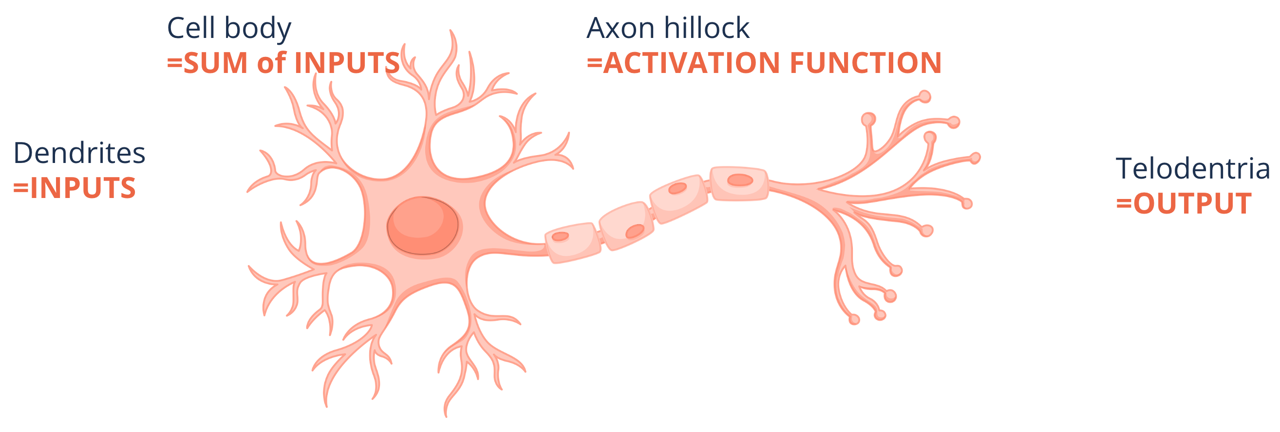
“one learning algorithm” hypothesis - plug in any sensor and given enough time the brain will learn to deal with it
How it ended#
A logistic unit
show_graph_visualization("../images/neural_networks/nn_2layers.gv")

How it ended#
A logistic unit with a bias term
ACTIVATION FUNCTION -
for example sigmoid
show_graph_visualization("../images/neural_networks/nn_2layers_bias.gv")

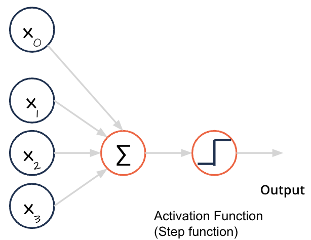
A different neuron: the Perceptron#
Input and output are numbers
Each input is associated with a weight
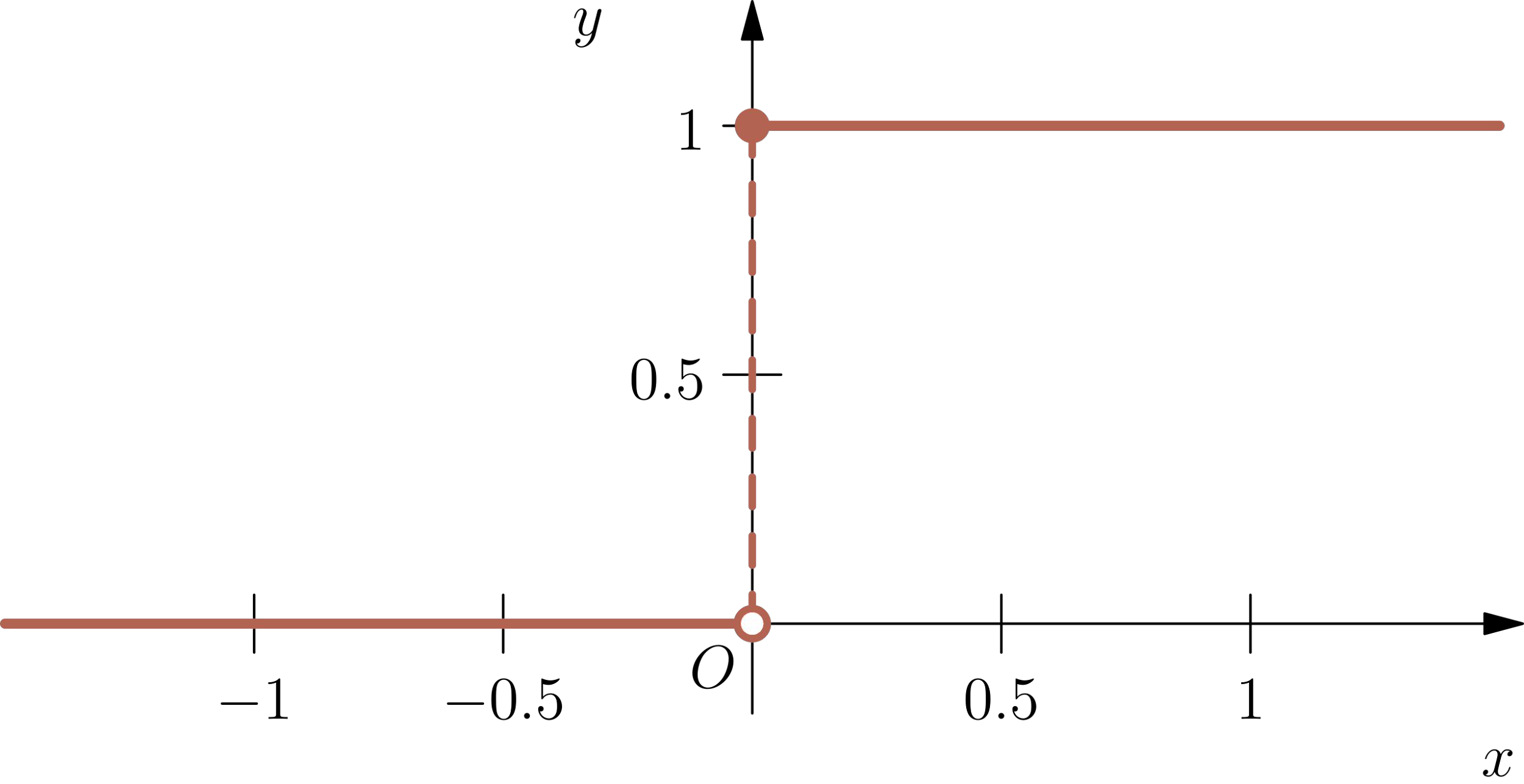
Example step function:
\( s t e p(z)=h e a v i s i d e(z)=\left\{\!\!\begin{array}{c c}{{0}}&{{z<0}}\\ {{1}}&{{z\ge0}}\end{array}\right.\)
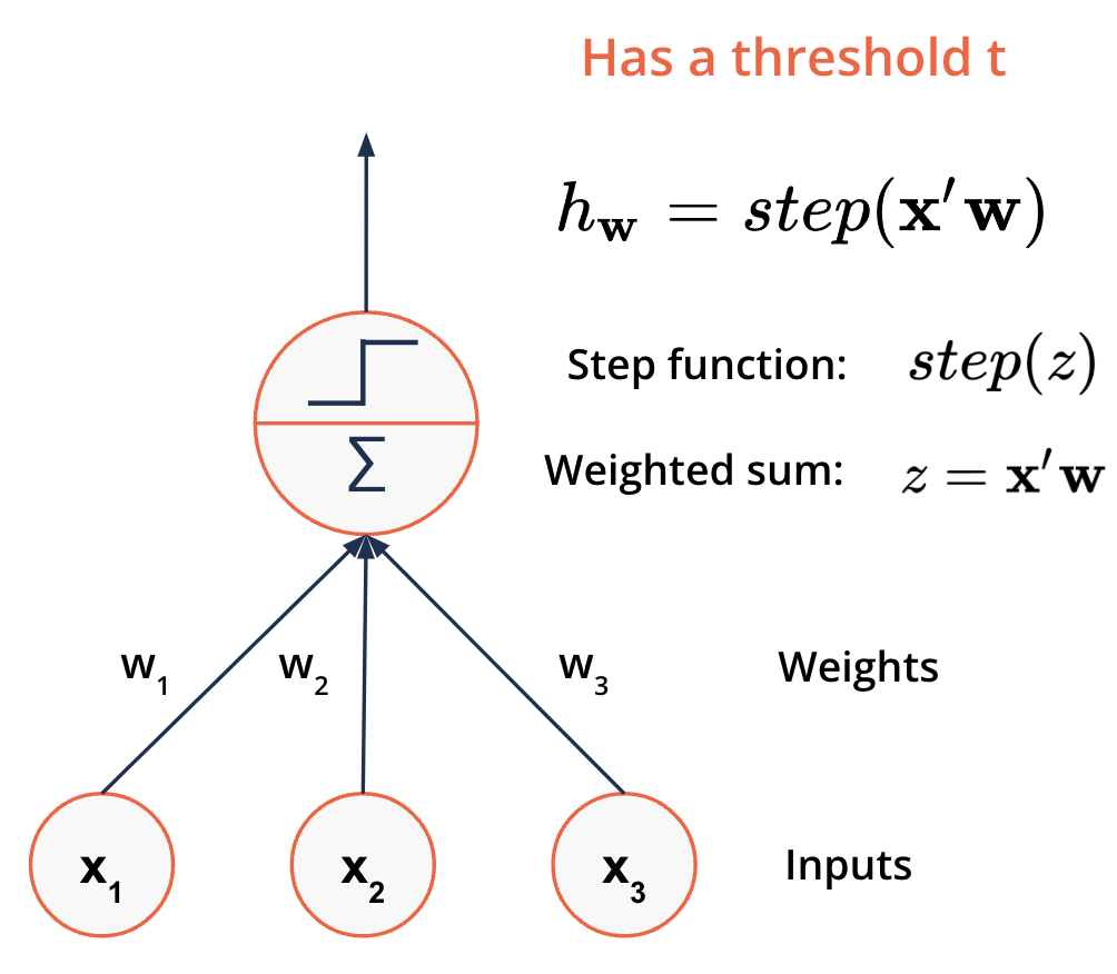
Rosenblatt, F. (1958), “The Perceptron: A Probabilistic Model for Information Storage and Organization in the Brain”
Activation Function#
In the first Perceptron a step-function was used.
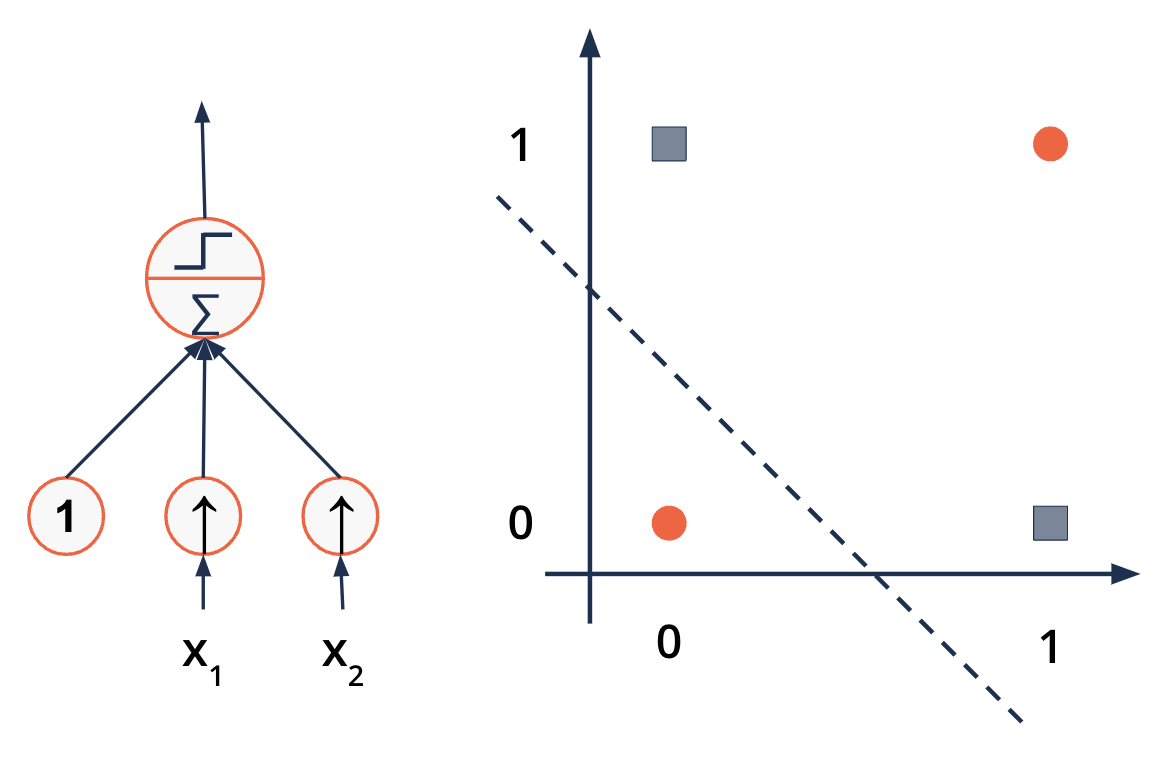
The XOR problem - the end of the Perceptron#
Exclusive OR: (\(x_1\) OR \(x_2\) are 1 but never both)
Perceptron fails at this simple problem
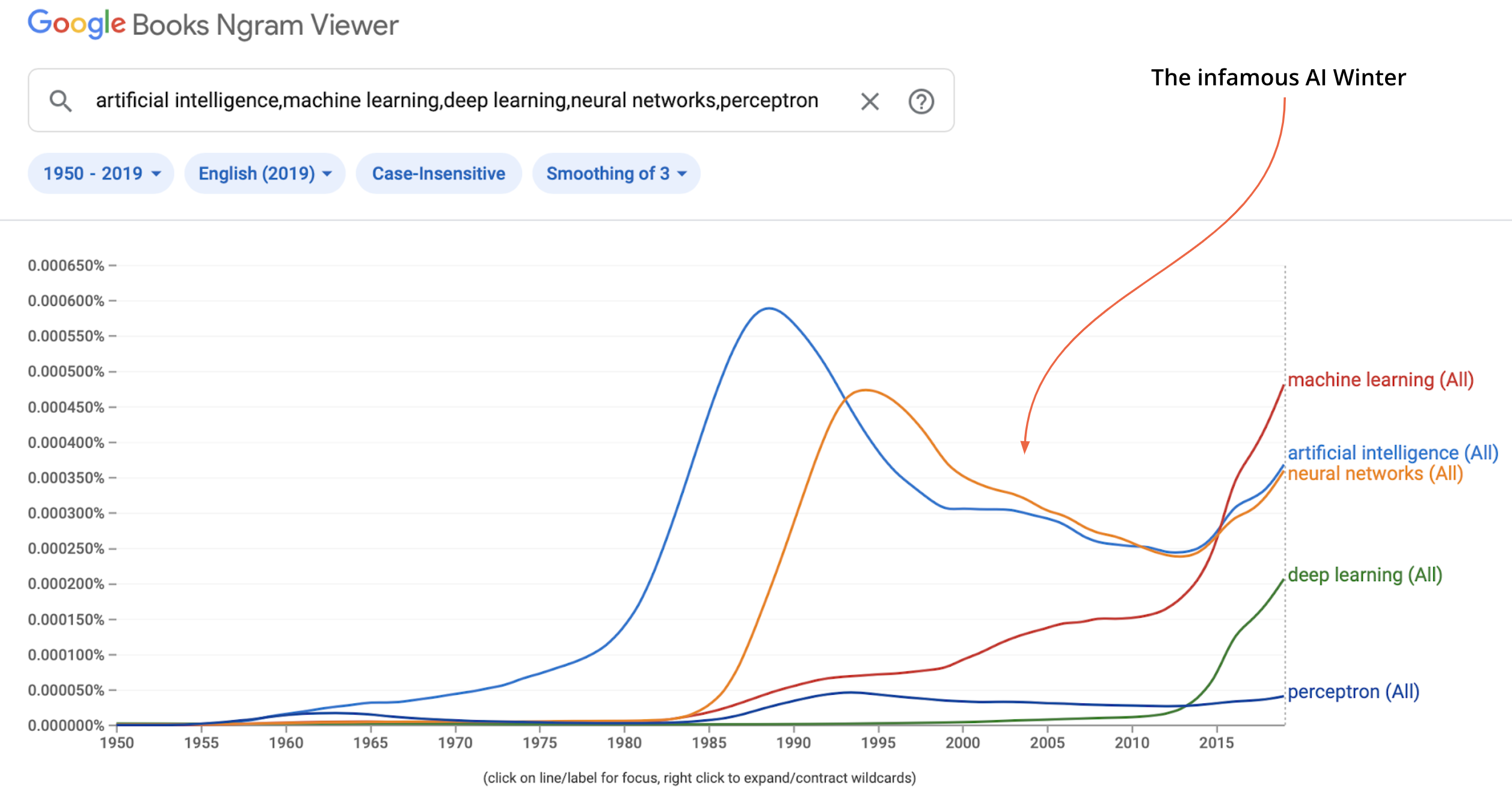
One of the reasons for the first AI Winter (1973)
https://towardsdatascience.com/perceptrons-logical-functions-and-the-xor-problem-37ca5025790a
The XOR problem - the end of the Perceptron#
Exclusive OR: (\(x_1\) OR \(x_2\) are 1 but never both)
Perceptron fails at this simple problem
One of the reasons for the first AI Winter (1973)
x1 |
x2 |
Output |
|---|---|---|
0 |
0 |
0 |
0 |
1 |
1 |
1 |
0 |
1 |
1 |
1 |
1 |
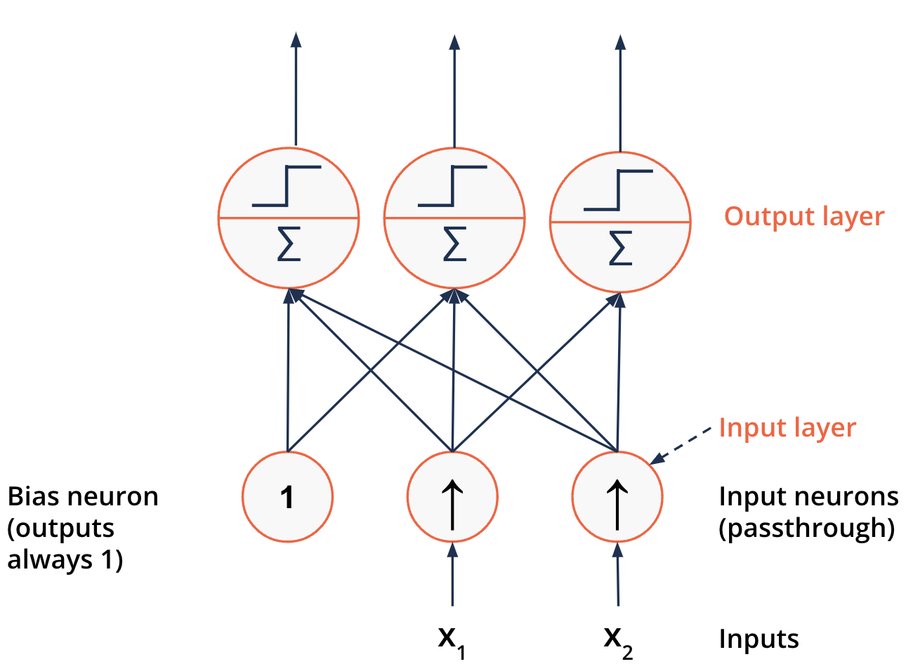
Logical computations and neurons#
More than one possible outcome - more Perceptrons
Here: three possible outcomes
Described as a {fully connected layer} or {dense layer}
Logical computations and neurons#
The XOR problem - the end of the Perceptron
Two Lines are needed to separate the classes
Two Perceptrons could solve this
But two binary outputs
Two outputs with three combinations: [00, 10, 11]
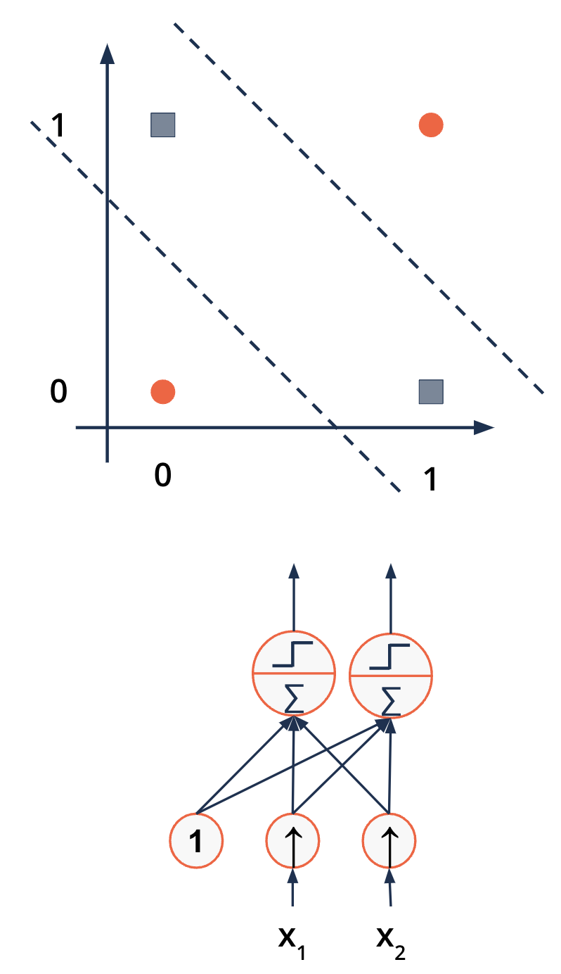
Minsky, M. and Papert, S. (1969): “Perceptrons: An Introduction to Computational Geometry”
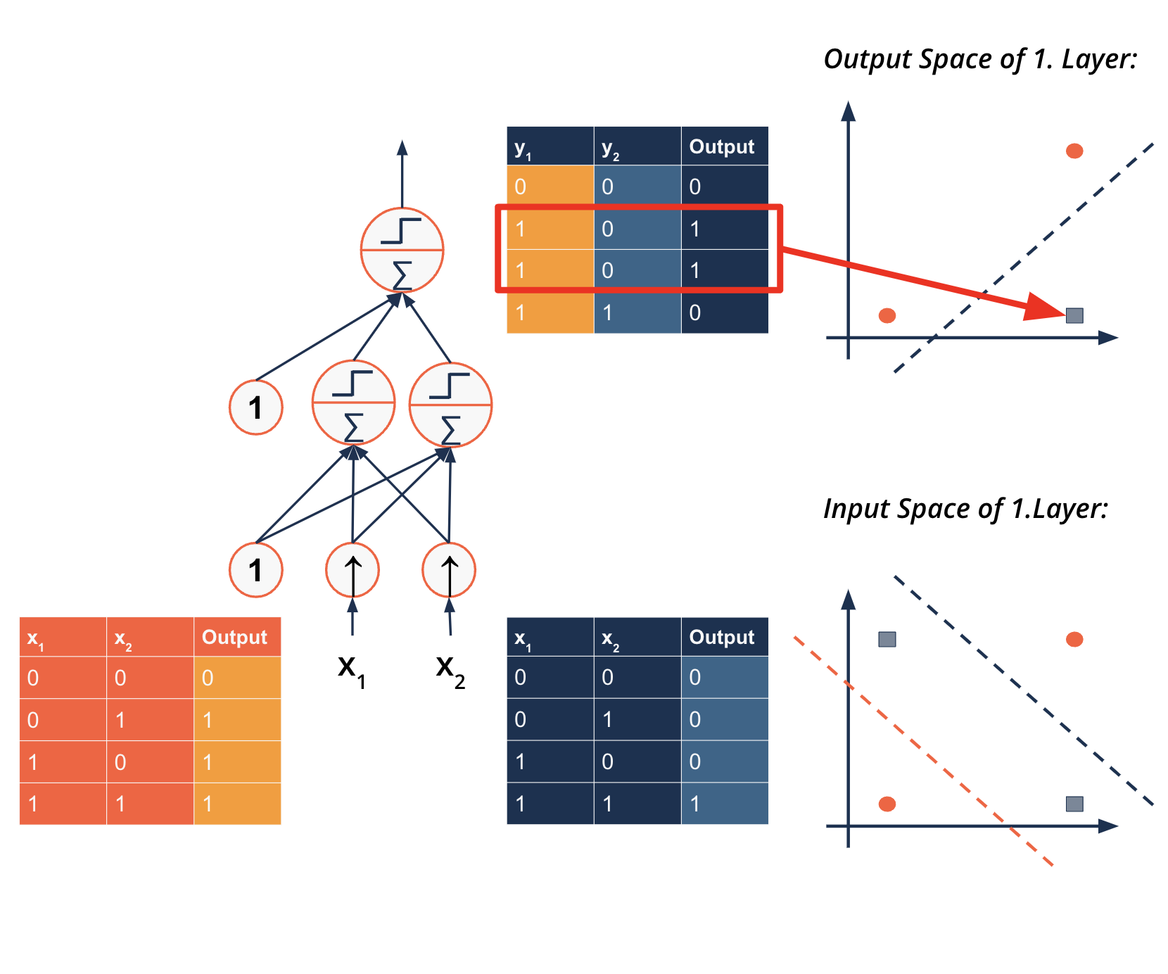
Logical computations and neurons#
The XOR problem - a multilayer problem
Adding a second layer solves the XOR problem
Multilayer Perceptron (MLP)
Breaks problem into sub-problems
Solves sub-problems
Combines results
The Neural Network#
Neural network#
show_graph_visualization("../images/neural_networks/nn_3layers.gv")

Neural network#
layer 0 = input layer
layer 1 = hidden layer (can be more of course)
layer 2 = output layer
show_graph_visualization("../images/neural_networks/nn_3layers_bias.gv")

Neural network#
show_graph_visualization("../images/neural_networks/nn_3layers_bias.gv")
Neural network#
j is the layer number
How many dimensions does W for j =1 have?
show_graph_visualization("../images/neural_networks/nn_3layers_bias.gv")
In ‘numpy notation’:
\(\begin{align} W^{(j)}\text{.shape} &= \left(\text{size}_{j+1} , (\text{size}_j + 1)\right)\\ &=(3,4)\\ \end{align}\)
Deep Neural Networks and compact representations#
What Network architecture can solve the Parity function:
Here for D=4:
Deep Neural Network with a single hidden layer: 55 neurons required to solve the problem

Deep Neural Network with D=4 hidden layers: 16 neurons required to solve the problem (much more compact as size is linear)

Deep learning and parameter search#
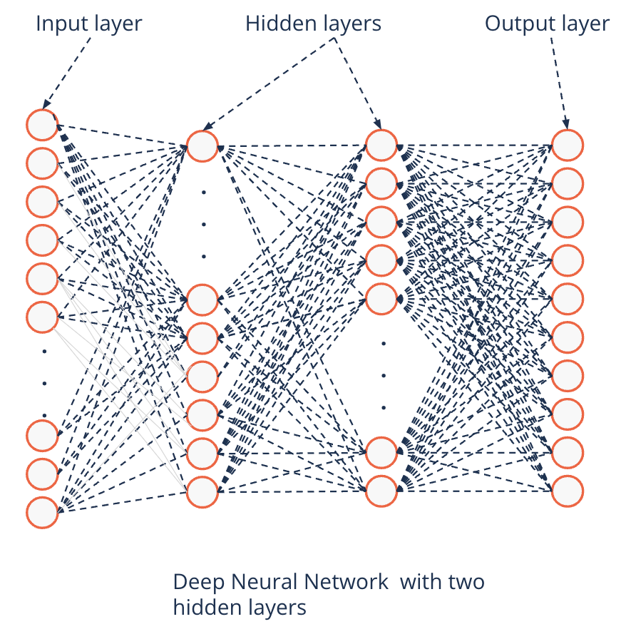
Deep Neural Networks
Deep neural networks
At least one hidden layer
Can theoretically approximate any function
Universal Approximation Theorem (Hornik (1991))
With arbitrary activation functions
Even with only a single hidden layer
Why than deeper?
Cybenko, G. (1989), “Approximation by Superpositions of a Sigmoidal Function”
Hornik, K. (1991), “Approximation Capabilities of Multilayer Feedforward Networks”
Csáji, B.C., (2001), “Approximation with Artificial Neural Networks”
Training the network#
Deep learning and parameter search#
How to find the parameters?
First intuition: Gradient descent
But how to apply the algorithm with many coupled and nested functions?
Backpropagation was a breakthrough in research
Makes training of very deep networks possible
Error is backpropagated through a network (End to Begin)
Gradient is calculated step-wise
Problem: Gradient of the step function is almost always zero
What now?
Werbos, P.J. (1974), “Beyong Regression: New Tools For Prediction And Analysis In The Behavioral Sciences”
Linnainmaa, S. (1970), “The representation of the cumulative rounding error of an algorithm as a Taylor expansion of the local rounding errors”
Rumelhart, D., Hinton, G. and Williams, R. (1986), “Learning Internal Representations by Error Propagation”
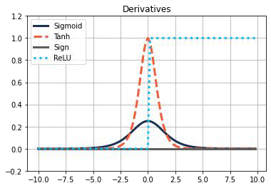
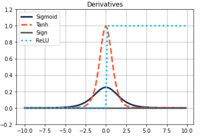
Non-linear activation functions#
Make Backpropagation possible
Gradient at almost any point in space
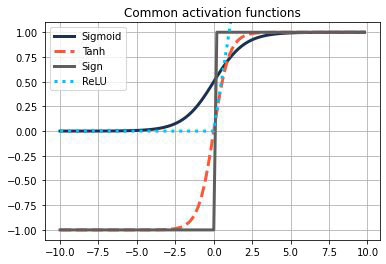
Most common activation functions are
Sigmoid \(\hspace{0.5cm} \sigma(z) = \frac{1}{1+\exp{(-z)}}\)
Tanh \(\hspace{0.5cm} \tanh(z) = \frac{\exp{(z)} - \exp{(-z)}}{\exp{(z)}+ \exp{(-z)}}\)
ReLU (Rectified Linear Unit) \(\hspace{0.5cm} ReLU(z) = \max(0,z)\)
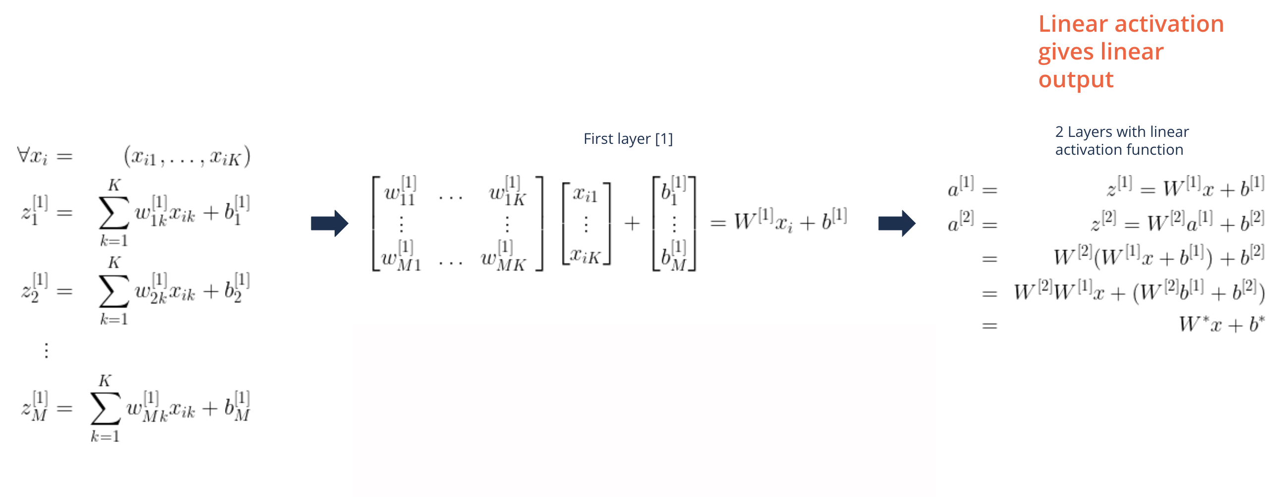
Non-linear activation functions#
Non-linear activation functions are needed to model more interesting output function
Linear activation functions give linear models
Linear activation functions can be used in Regression problems
Hidden layers should be non-linear nevertheless
Hidden layers with linear activation functions and a sigmoid output:
Logistic regression
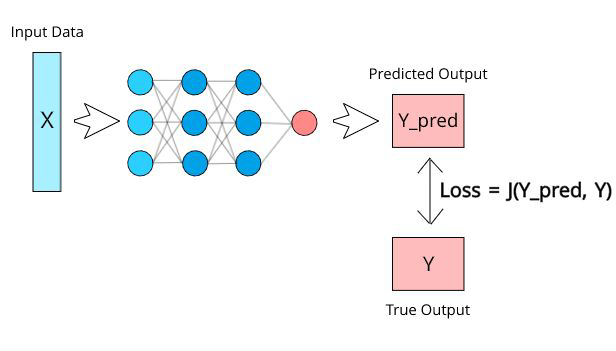
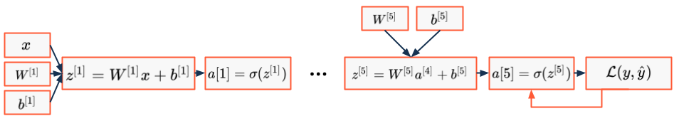
Feed-forward step#
In the feed-forward step the data is propagated through the network from input to output
show_graph_visualization("../images/neural_networks/feed-forward-step.gv")

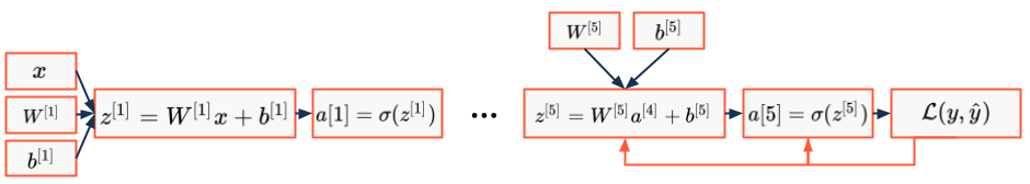
Back-propagation#
How can we discover in which direction and with which magnitude to tweak the parameters?
We do the same as usual: Start at the loss function

Binary Loss (like in Logistic regression):
show_graph_visualization("../images/neural_networks/back_prop.gv")

Feed forward and back propagation#
Back prop - intuition#
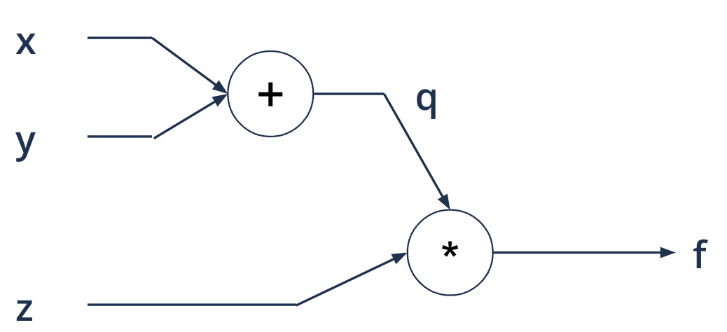
Computational graphs#
A directed graph where the nodes correspond to mathematical operations
\(f(x, y, z) = q * z = (x + y)*z\)
Computational graphs - feed forward#
Going left to right
\(f(x, y, z) = (x + y)*z\) eg. \(x = 1, y = 3, z = -3\)
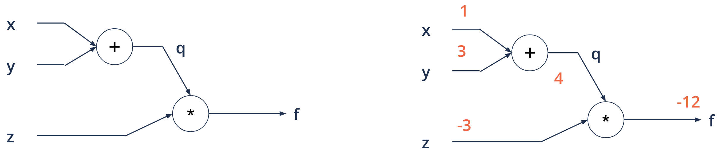
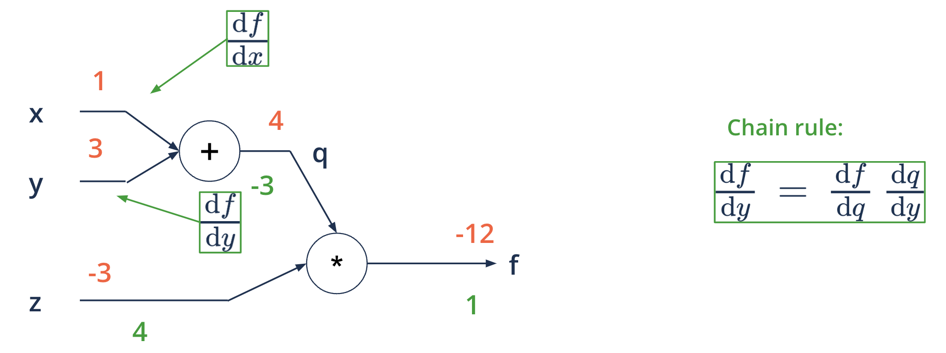
Computational graphs - backward propagation#
Objective: compute gradients for each input with respect to the output, to use in gradient descent
\(f(x, y, z) = (x + y)*z\) eg. \(x = 1, y = 3, z = -3\)
Backward propagation#
going from right to left
\(f(x, y, z) = (x + y)*z\) eg. \(x = 1, y = 3, z = -3\)
Backward propagation#
going from right to left
\(f(x, y, z) = (x + y)*z\) eg. \(x = 1, y = 3, z = -3\)
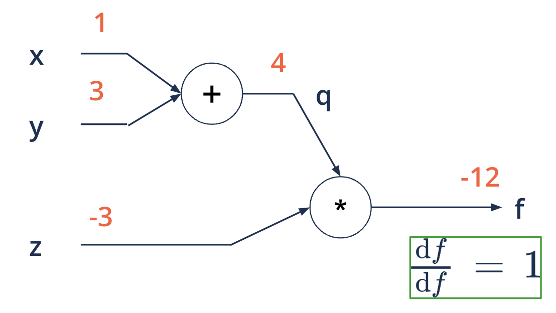
Backward propagation - starting at the end#
applying the chain rule of differentials
\(f(x, y, z) = (x + y)*z\) eg. \(x = 1, y = 3, z = -3\)
Backward propagation - starting at the end#
applying the chain rule of differentials
\(f(x, y, z) = (x + y)*z\) eg. \(x = 1, y = 3, z = -3\)
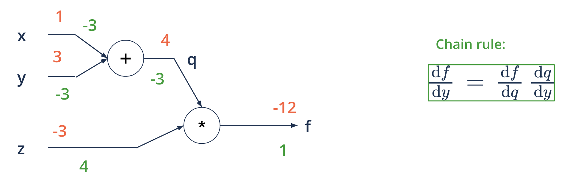
Backward propagation - starting at the end#
applying the chain rule of differentials
\(f(x, y, z) = (x + y)*z\) eg. \(x = 1, y = 3, z = -3\)
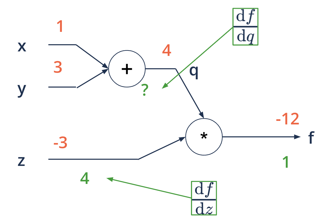
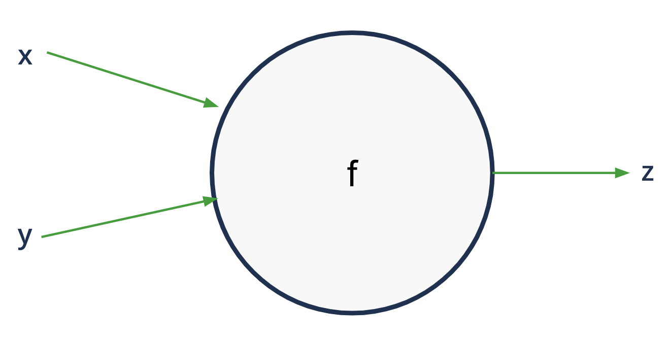
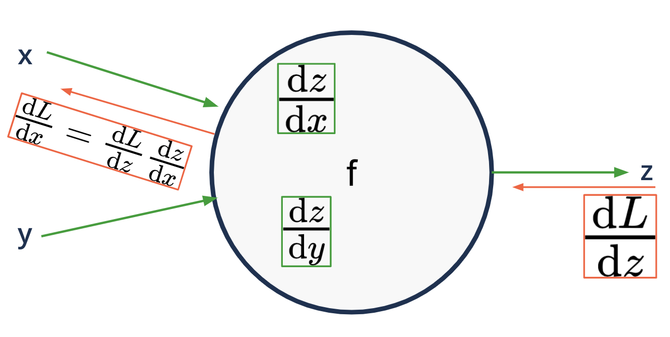
Backward propagation#
each node is aware of its surroundings
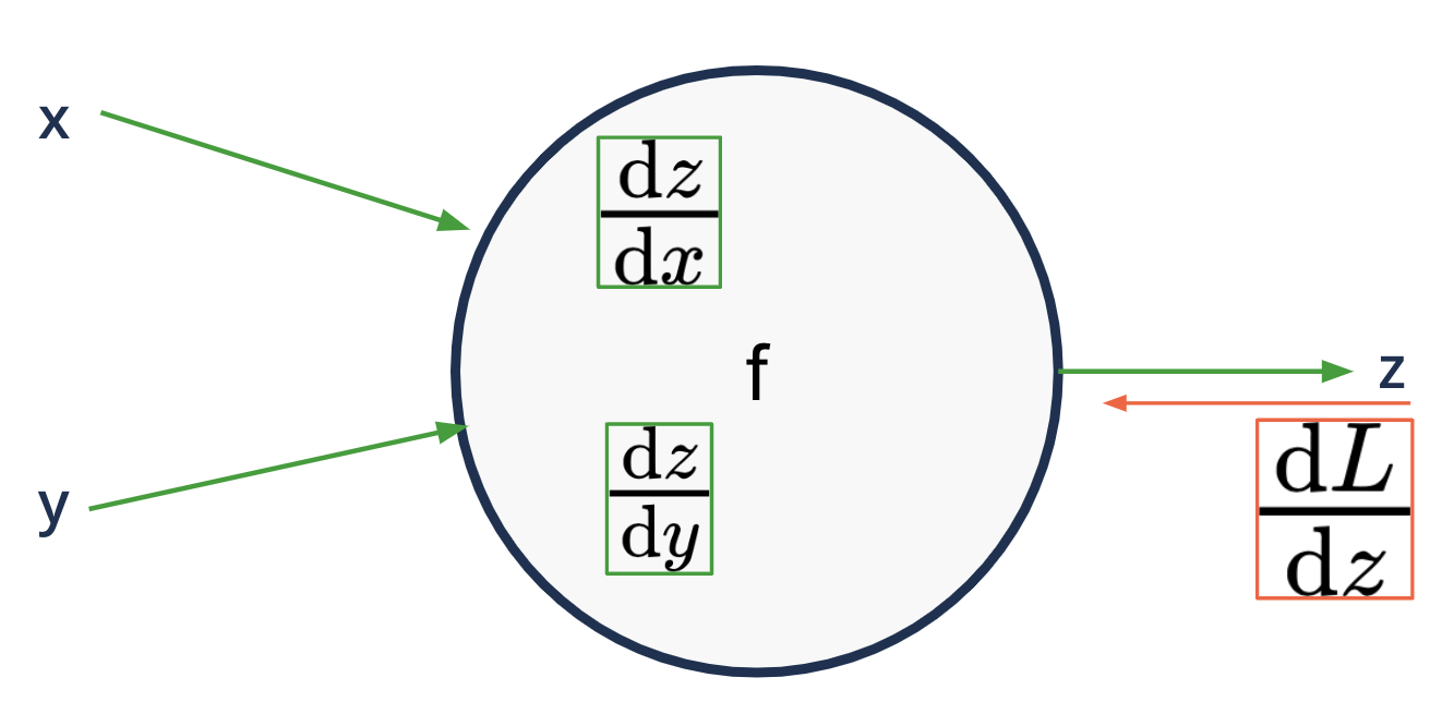
Backward propagation#
each node is aware of its surroundings
and we know the local gradients - easy to compute (z is usually a
simple operator: sum, product, exp..)
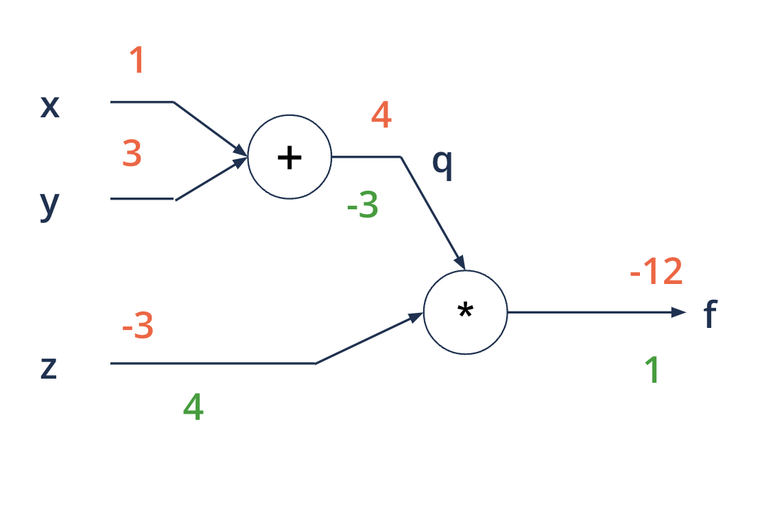
Backward propagation#
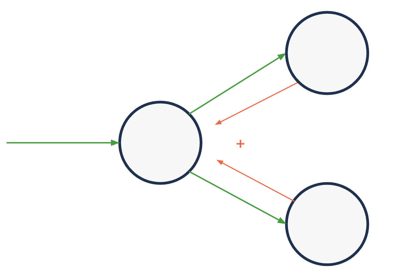
applying the chain rule
Backward propagation#
gradients add at branches
Back prop - math#
Back-propagation for binary loss#
Binary Loss (like in Logistic regression):
show_graph_visualization("../images/neural_networks/back_prop.gv")
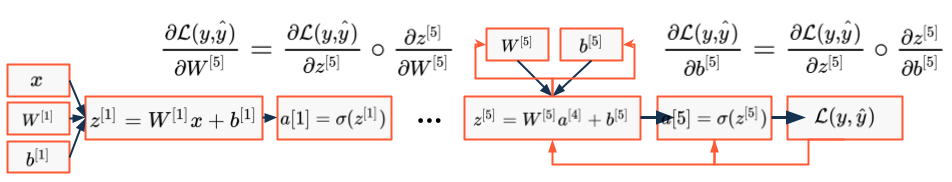
Back-propagation#
- To get the derivation of loss towards the parameters:
- Consider the {computation graph}
- Start at the end and derive

Back-propagation#
- Then, take the next step backwards in the graph
- Compute the derivation towards the neurons

show_graph_visualization("../images/neural_networks/back_prop_step_1.gv")

Back-propagation#
- To get to the derivation for the last parameters
- Derive the neuron towards its parameters
show_graph_visualization("../images/neural_networks/back_prop_step_2.gv")

Back-propagation#
- Repeat and step back towards the first layer ...
- ... and its parameters
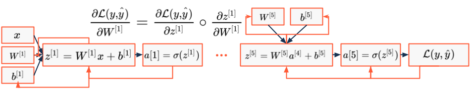
show_graph_visualization("../images/neural_networks/back_prop_all_steps.gv")

Back-propagation#
- Now we have the direction for the parameter update
- As usual learning rate gives step-size
- Make the parameter update:
- Start again with the {feed-forward} step ...
- ... and iterate
- ... and iterate

Feed forward and back propagation#
Training deep neural networks#
- Backpropagation enabled researchers to train neural networks in a single algorithm
- Before layerwise training had been used
- However, networks with a large number of layers still had problems
- Vanishing/exploding gradients

Vanishing/Exploding gradients#
- First approaches to train deep networks with backpropagation failed
- Gradients were becoming very small or very large during training
- Vanishing: direction for parameter update unknown
- Exploding: training becomes unstable
- Gradients were becoming very small or very large during training
- Hochreiter (1991) formalized the problem in his Diploma thesis
- Since then the problem was examined extensively
- Many approaches have since been developed to tackle the problem
Hochreiter, S. (1991), “Untersuchungen zu dynamischen neuronalen Netzen”
Pascanu, R., Mikolov, T. and Bengio, Y. (2013), “On the difficulty of training Recurrent Neural Networks”
Vanishing/Exploding gradients#
- Many layers intensify unbalanced parameter values
- Holds as well for gradients in backward propagation
- Initialization is crucial
- Well balanced parameters help
- Xavier - Tanh
- He - ReLU
- Activation functions can have zero or almost zero gradients
- Use ReLU - saturates only in one direction
activation: linear
\( \hat{y}=W^{[1]}\cdot W^{[2]}\cdot\cdot\cdot W^{[L]}x\)
\( W^{[l]}=\begin{bmatrix}1.5 & 0\\ 0 & 1.5\end{bmatrix}\)
Glorot, X., Bordes, A. and Bengio, Y. (2010), “Deep Sparse Rectifier Neural Networks”
Glorot, X. and Bengio Y. (2010), “Understanding the difficulty of training deep feedforward networks”
He, K. et al. (2015), “Delving deep into rectifiers: Surpassing human-level performance in ImageNet classification.”
Sussillo, D. and Abbott, L.F. (2015), “Random Walk Initialization For Training Very Deep Feedforward Networks”
Mishkin, D. and Matas, J. (2016), “All you need is a good init”
Buliding your own NN#
Hyperparameters#
Hyperparameters#
- What hyperparameters exist?
- Learning rate - very important
- Number of layers - not so much
- Number of neurons per layer - important
- Number of features - important
- Mini-batch size - important
- Optimization algorithm - important
- Learning rate decay - not so much
- How to tune them?
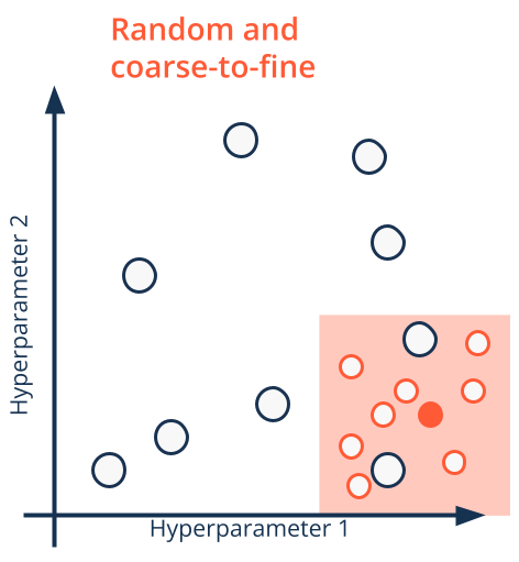
- Try random values - do not use a grid!
Search Strategies#
- Hyperparameter search in neural networks underlies curse of dimensionality
- Many parameters to tune
- Unknown which are the important ones for the problem
Search Strategies#
- Hyperparameter search in neural networks underlies curse of dimensionality
- Many parameters to tune
- Unknown which are the important ones for the problem
- Usually it is used an approach based on
- Random search
- Coarse-to-fine
- Well-scaled (often log-scaled)
Regularization#
Regularization#
- L2 Regularization:
\( ||w||_{2}^{2}=\sum_{j=1}^{m}w_{j}^{2}=w^{T}w \)
- L1 Regularization:
\( ||w||_{1}=\sum_{j=1}^{m}|w_{j}| \)
Regularization#
- L2 Regularization:
\[ ||w||_{2}^{2}=\sum_{j=1}^{m}w_{j}^{2}=w^{T}w\]
- L1 Regularization:
\[ ||w||_{1}=\sum_{j=1}^{m}|w_{j}|\]
- L2 Regularization:
\[||W^{[l]}||_{F}^{2}=\sum_{j=1}^{n_{[l-1]}}\sum_{i=1}^{n_{[l]}}(w_{i j}^{[l]})^{2}\]
- L1 Regularization:
\(\scriptsize J(w,b)=\frac{1}{m}\sum_{i=1}^{m}\mathcal{L}(\hat{y}_{i},y_{i})+\frac{\lambda}{2m}||w||_{2}^{2}+\underbrace{\frac{\lambda}{2m}b^{2}}_\text{negligible impact}\)
\(\scriptsize J(W^{[1]},b^{[1]},\cdot\cdot\cdot,W^{[L]},b^{[L]})=\frac{1}{m}\sum_{i=1}^{m}\mathcal{L}(\hat{y_{i}},y_{i})+\frac{\lambda}{2m}\sum_{l=1}^{L}|W||_{F}^{2}\)
The effect of sub-networks#
- Why does L2 regularization prevent overfitting in neural networks?
- Intuitively: it creates a simpler network
- Many parameters will be turned very small
- Signals flow mainly via some few routes through the network

Extreme L2 Regularization:
show_graph_visualization("../images/neural_networks/l2_regularization.gv")

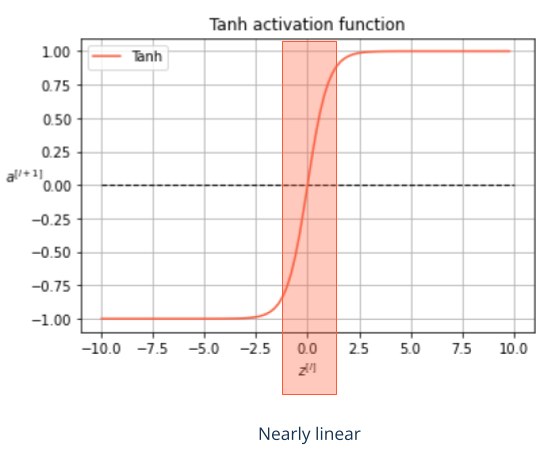
The effect of mid-range activation functions#
- What role play activation functions in L2 regularization?
- Non-linear activation functions possess nearly-linear parts
- Sufficiently small parameter values enforce small inputs
- In this definition range many activation functions are near to linear
- As a result the network itself is forced to become nearly linear
- Variance shrinks and bias increases

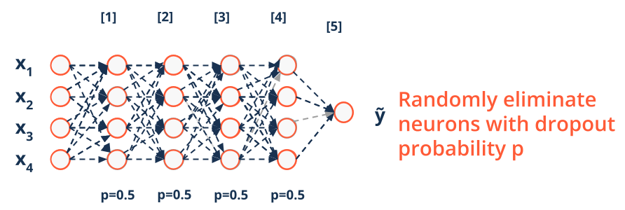
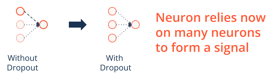
Regularization techniques in deep learning - Dropout#
- Dropout is a very powerful regularization method for neural
networks
- Randomly eliminate nodes in each optimization step
- Dropout prevents units from co-adapting
Srivastava et al. (2014), “Dropout: A Simple Way to Prevent Neural Networks from Overfitting”
Regularization techniques in deep learning - Intuitive explanation to neural co-adapting#
- A single neuron relies on the input of its predecessor neurons
- Bears the risk of relying on a few predecessors that activate on noise
- Dropping neurons randomly then forces the neuron to diversify
- Each predecessor signal could vanish with dropout

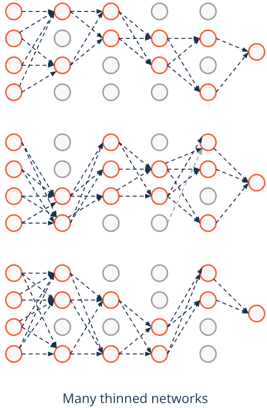
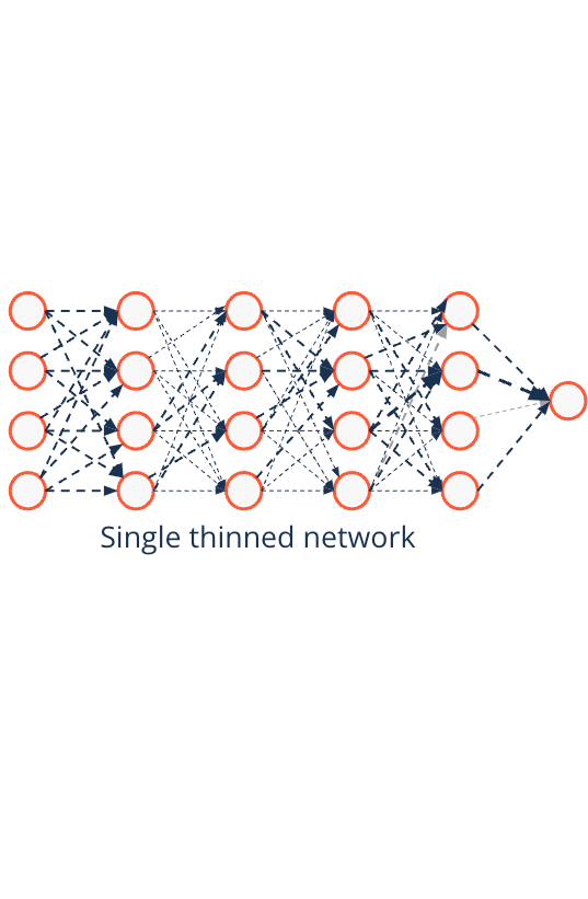
Regularization techniques in deep learning - Dropout mimics ensembling#
- Instead of testing many different networks by training each of them in isolation
- Dropout tests them during a single optimization
- Predictions are approximating the average over all thinned networks
- This is similar to ensemble learners
- In contrast to ensembles effect is reached by using unthinned network with smaller weights
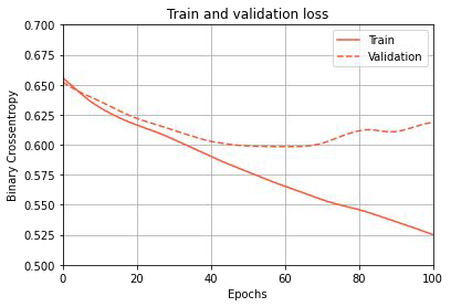
Regularization techniques in deep learning - Early stopping can be resourceful#
- Early stopping is used to find the optimal point
- Validation error raises again
- Builds on the development of weights during training
- Weights start small and increase
- Not the best method to regularize
- Orthogonalization of optimizing and regularizing gets lost
Wang et al. (1994), “Optimal Stopping and Effective Machine Complexity in Learning” Caruana et al. (2001), “Overfitting in Neural Nets: Backpropagation, Conjugate Gradient, and Early Stopping”
Frameworks#
Python deep learning libraries - Deep learning frameworks#
- There exist a couple of major deep learning libraries
- TensorFlow is the one most used in production
- Since TensorFlow version 2.0 Keras is part of TensorFlow
- Keras is an high-level API to TensorFlow
- Abstracts away a lot of complexity in coding
- Ease the building and training of models by
- modules for layers, optimizers and activation functions
- parallelized training processes


Python deep learning libraries - TensorFlow and Keras#
- We focus on TensorFlow and use Keras
- Well maintained and highly active development
- Most relevant in business
- TensorFlow works with a directed acyclic computation graph (DAG)
- Programmable in Python
- Gets compiled in C++ and is very fast
- Tensors flow through the DAG
Abadi et al. (2015), “TensorFlow: Large-Scale Machine Learning on Heterogeneous Distributed Systems”
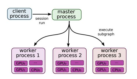
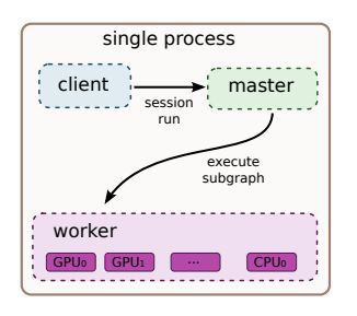
Python deep learning libraries - The power of TensorFlow#
- Enables deep learning
- of very large and deep models
- on massive data sets
- Possible via distributed systems with special hardware
- Subgraphs are placed on different devices
- Send/Receive nodes communicate across workers
- Fault tolerance is ensured by
- monitoring communication between processes
- re-executing when errors are detected
- saving checkpoints for economic restarts
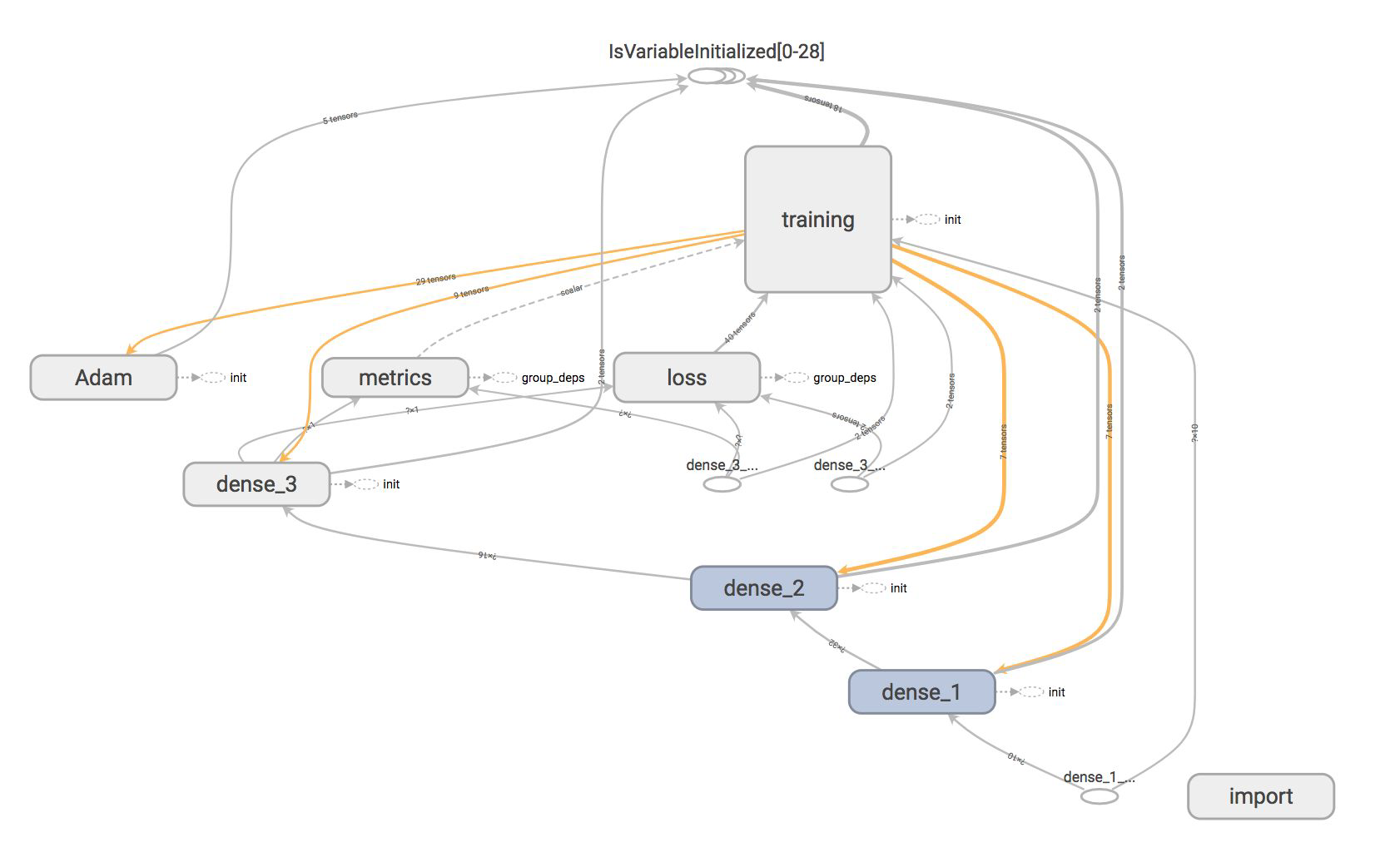
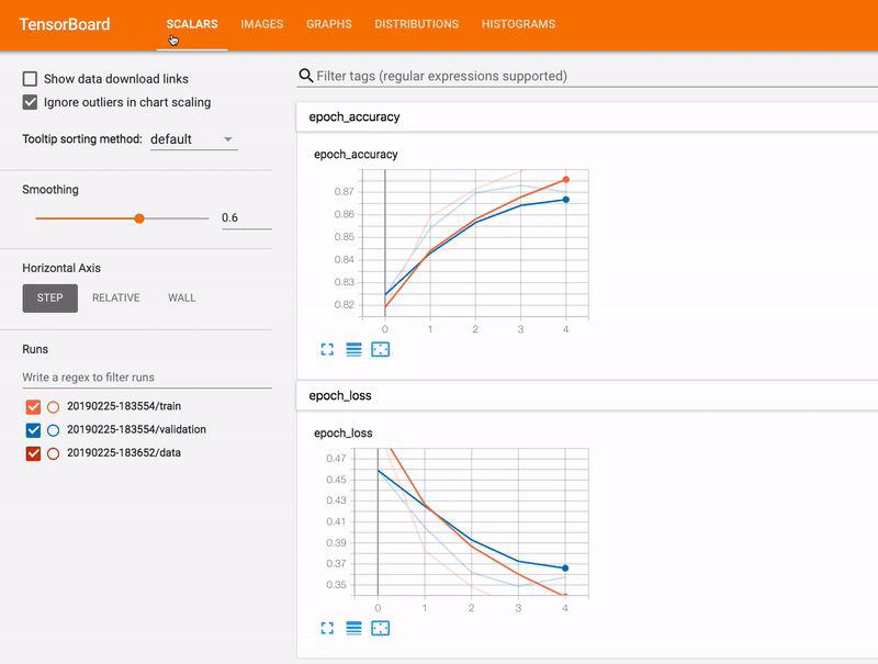
Python deep learning libraries - TensorBoard - TensorFlow visualization#
References#
Rosenblatt, F. (1958), “The Perceptron: A Probabilistic Model for Information Storage and Organization in the Brain”
Minsky, M. and Papert, S. (1969): “Perceptrons: An Introduction to Computational Geometry”
Lighthill, J. (1972), “Artificial Intelligence: A General Survey”
https://cs231n.github.io (stanford course notes)