Linear Regression#
Motivation#
Goals of Linear regression#
I own a house in King County!
It has 3 Bedrooms, 2 Bathroom, a nice 10.000 sqft lot and is only 10km away from Bill Gates mansion!
If only I had a way of estimating what it is worth…

If only I had a way of estimating what it is worth…#
Use training data to …
… find a similar house …
… and use its value for estimation.
Use training data to …
… find a general rule that …
… can be used for estimation.
I should train a Regression Model!#
    216.645 $ Basis-price

+   20.033 $ for each bedrooms

+  234.314 $ for each bathrooms

+        1 $ for each sqft lot

-   14.745 $ for each km distance from Bill Gate Mansion

= xyz $ estimated house price
The term regression (e.g. regression analysis) usually refers to linear regression.
(Don't confuse with logistic regression.)
Building a model#
Descriptive statistics
Using LR for explanation (profiling)→ Why is my house worth xyz?
→ How can I increase the price?
Inferential statistics
Using LR to make predictions→ How much is my house worth?

Notes: There are two methods in statitics:
descriptive (→ EDA) and
inferential (→ ML)
Linear Equation#
Linear Equation#
Q: What is the equation of the line?#
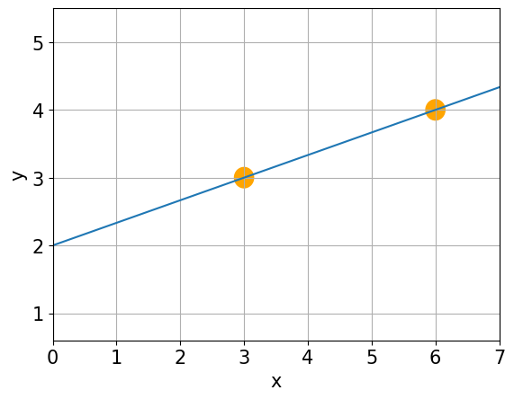
Linear Equation#
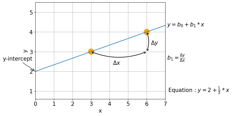
Intercept (b0, value of y when x = 0)
Slope (b1, weights)
Linear Regression#
Linear Regression#
Is the variable X associated with a variable y, and if so,
what is the relationship and can we use it to predict y?
Correlation — measures the strength of the relationship → a number
Regression — quantifies the nature of the relationship → an equation
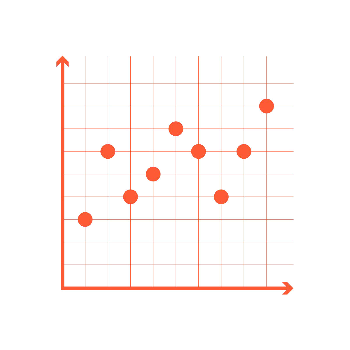
What about more than 2 points?#
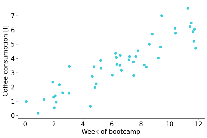
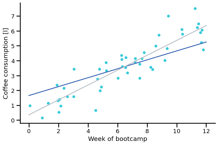
Let’s look at an example#
Two correlated variables:
week of bootcamp, \(x\)
coffee consumption, \(y\)
\(r=0.9\)
\( y=b_{0}+b_{1}\cdot x+e\)
→ Find \( b_0 \) and \( b_1 \) !
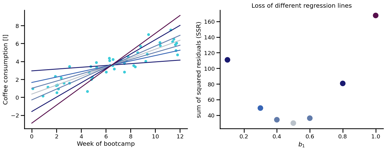
Trying out some lines. Which one is better?#
Grey: \( \hat{y} = 0.35 + 0.5 \cdot x \)
Blue: \( \hat{y} = 1.65 + 0.3 \cdot x \)
^ - the “hat” notation means the value is estimated (the lines) as opposed to a known value (the dots).
The estimate has uncertainty (!) whereas the true value is fixed.
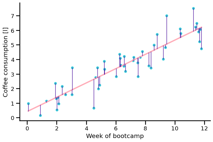
How do we know which line is better?#
Residuals#
\(e_i = y_i - \hat{y}_i\)
which means:
\(y_i = b_0 + b_1 \cdot x_i + e_i\)
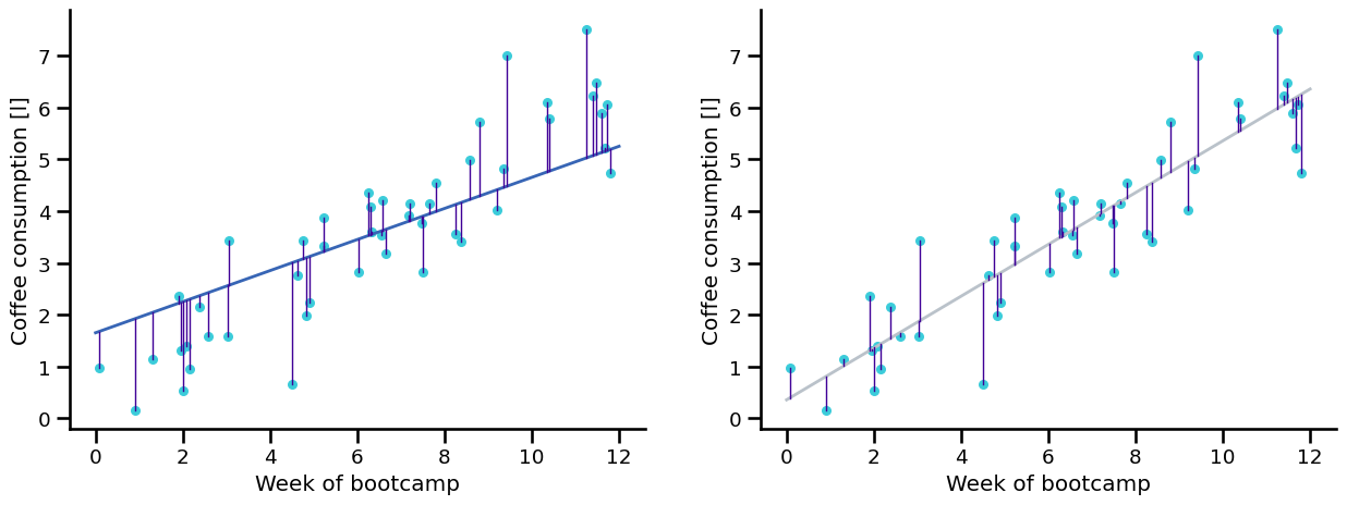
Least squares criterion#
By comparing the sum of squared residuals (SSR) we can find out which one is better:
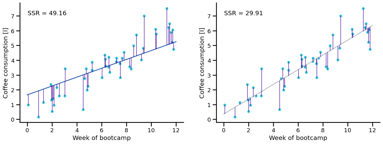
Trying out several fitted lines#
By comparing the sum of squared residuals (SSR) we can find out which one is better:
BUT THERE CAN BE AN INFINITE NUMBER OF LINES!#
So how do we do this?#
Obviously doing it manually is not really scalable
We minimize the OLS-function \(J(b_0 , b_1 )\) with respect to \(b_0\) and \(b_1\)!
OLS - Ordinary Least Squares
Ordinary least squares regression#
we divide the first equation by 2n:
… more math leads to:
Fun facts about residuals#
The second equation means the error/residual is uncorrelated with the explanatory variable
feel free to try this out for your models
Model performance#
Mean \(\bar{y}=\frac{1}{n} \sum\limits_{i=1}^{n}y_{i}\)#
Variance \(\sigma^2 = \frac{1}{n-1}\sum_i{(y_i-\bar{y})^2}\)#
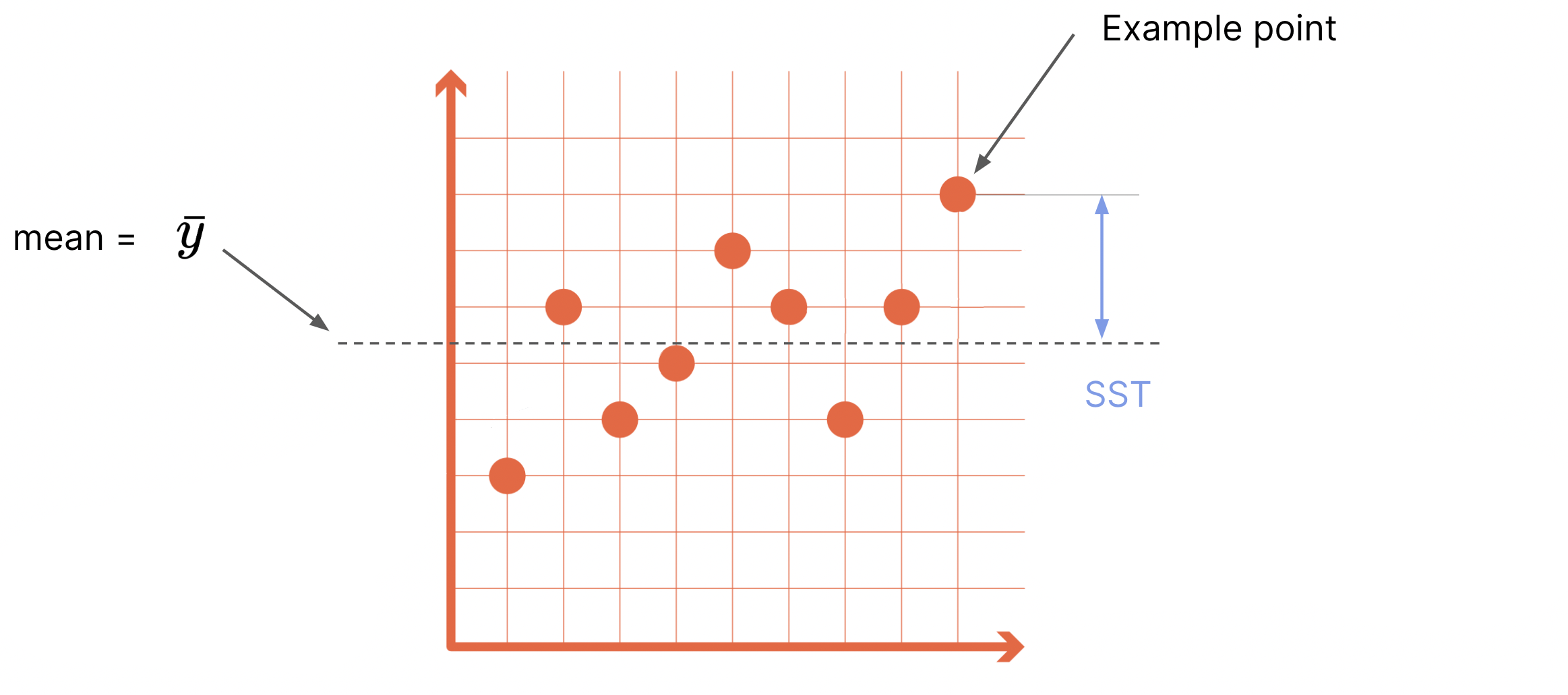
Sum of various squares (variance analysis)#
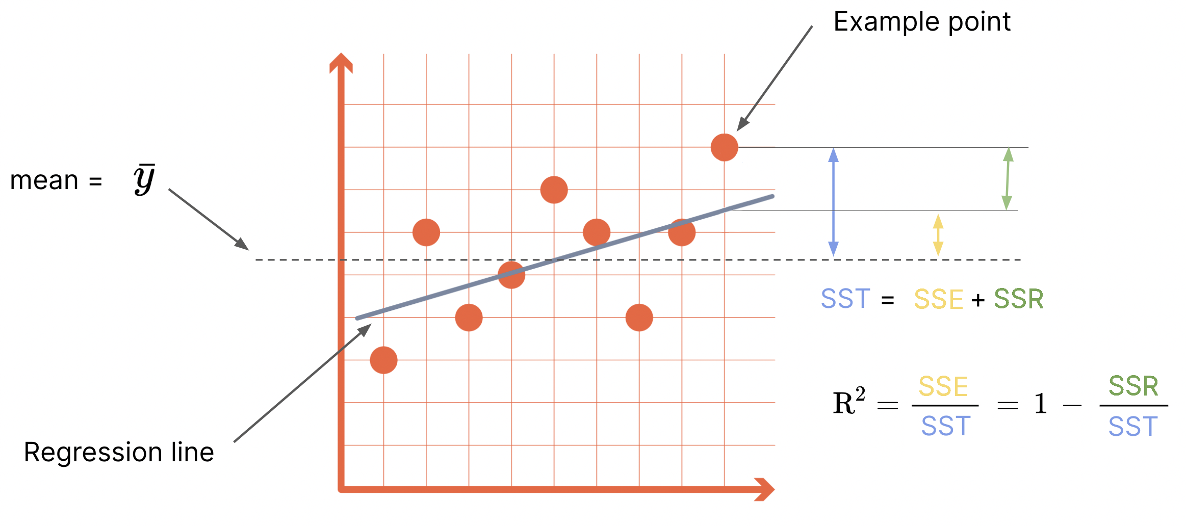
SST = total sum of squares
SSE = explained sum of squares
SSR = remaining sum of squares
\(0 ⪯ R^2 ⪯ 1\)
least squares criterion ~ maximizing R2
\(R^2= r^2\)( you know.. the Pearson correlation coefficient)
Root mean squared error#
The objective to fit the linear regression line is minimizing the sum of squared residuals (remarkable called MSE), this also optimizes the RMSE.
RMSE is also used to compare performance of other ML models.
Key Terms#
Key terms: Machine learning#
Variables:#
Target (dependent variable, prediction, response, y)
Feature (independent variable, explanatory/predictive variable, attribute, X)
Observation (row, instance, example, data point)
Model:#
Fitted values (predicted values) - denoted with the hat notation ŷ
Residuals (errors, e) - difference between reality and model
Least squares (method for fitting a regression)
Coefficients, weights (here: slope, intercept)
But I want to use more then one feature!#
Multiple LR#
Multiple regression#
So far we’ve dealt with only one feature. Every single observation follows this expression: \(y = b_0 + b_1x + e\).
Most of the time you will have many features.
A more general expression for all observations at once and any number of features translates to: \( y=X b+e \)
where y, b, e are vectors, and X is a matrix.
n= number of observations, m= number of features
\(x_{obs,feature} = x_{row,col} = x_{n,m}\)
\(y\) and \(X\) are known: They are the real data of all the observations.
\(b\) and \(e\) are not (yet) known.
The term multiple refers to the independant variable. A model which can predict several dependant variables at once is called multivariate linear regression model.
Normal Equation#
The optimal values for \(b\) (\(b_0\), \(b_1\), \(...\), \(b_m\)) will usually be calculated numerically using Gradient Descent method (topic of another lecture). However, they can also be determined analytically with the so-called normal equation:
Predictions#
Now as the \(b\) are also known (determind which whatever method), we can use them for making predictions.
$\( \hat{y} = b_0 + b_1x_1 + ... + b_mx_m \)$
Or in matrix notation:
\(X\) needs to be in the same format as the one used above but can have a different number of rows (e.g. only 1).
The error term \(e\) is unfortunately not known but has been minimized.
Multiple regression — evaluation metrics (special considerations)#
Root mean squared error (RMSE)#
Most widely used metric to compare models (also non-multiple regr.). It is a measure of the goodness of a model.
Disadvantage: The use of many (unnecessary) features leads to a (supposedly) good fit.
Adjusted R squared (\(adj. R^2\)):#
with n: sample size; p: number of explanatory variables of model
Modified version of R taking into account how many independent variables are used in the model.
Method: It penalizes the use of many features.
Overview of LR terms#
R: Pearson correlation coefficient — in the intervall between [-1, 1]
R²: Coefficient of determination — How much of the variance in the dependent variable is explained by the model
MSE: mean squared error — SSR divided by sample size
RMSE: root mean squared error — Metric to judge the goodness of a model; root of MSE
SST, SSE, SSR: Sum of squares: total, explained, remaining
\(\sigma^2\): Variance of a variable — Measure of dispersion from the mean of a set
Many of these terms are similar in meaning:
* Some refer to a set's mean while others refer to a model's prediction
* Some are divided by the sample size, while others are not or by the number of DoF
* By some of them the root is pulled, by others not
* In any case: SSR ↓ means RMSE ↓ means R² ↑ and vice versa
References#
There are also a lot of detailed explanations in the exercise repos.
Practical Statistics for Data Science - Peter Bruce & Andrew Bruce
Econometric Methods with Applications in Business and Economics - Christiaan Heij, Paul de Boer, Philip Hans Franses, Teun Kloek, Herman K. van Dijk
Difference between \(R^2\) and the adjusted version
Always welcome: Explation of LR by statquest
Some more math for those who want to know how to calculate \(b_1\)#
\(-2 \Sigma x_i(y_i - b_0 - b_1x_i) = 0 \)
we know that \(b_0 = \bar{y} - b_1 \bar{x}\)
\(-2 \Sigma x_i(y_i - \bar{y} + b_1 \bar{x} - b_1x_i) = 0 \)
\(\Sigma(x_iy_i - x_i \bar{y} + b_1(x_i \bar{x} - x_ix_i)) = 0\)
\(\Sigma(x_iy_i - 2x_i \bar{y} + \bar{x}\bar{y} + b_1(-\bar{x}\bar{x} + 2x_i \bar{x} - x_ix_i)) = 0 \hspace{1cm}|\hspace{1cm} \Sigma x_i = \Sigma \bar{x} \)
\(\Sigma(x_iy_i - x_i \bar{y} - \bar{x}y_i + \bar{x}\bar{y} + b_1(-\bar{x}\bar{x} + 2x_i \bar{x} - x_ix_i)) = 0 \hspace{1cm}|\hspace{1cm} \Sigma x_i \bar{y}= \Sigma \bar{x}y_i = n \bar{x}\bar{y} \)
\(\Sigma(y_i - \bar{y})(x_i - \bar{x}) - b_1 \Sigma(x_i - \bar{x})^2 = 0 \)
\(b_1 = \frac{\Sigma(y_i - \bar{y})(x_i - \bar{x})}{\Sigma(x_i - \bar{x})^2} \)