Unsupervised Learning - Dimensionality Reduction#
Unsupervised learning#
Statistical methods that extract meaning from data without training a model on labeled data
Unsupervised learning also constructs a model of the data but it doesn’t distinguish between target and predictor variables
finding groups of data → Clustering
reducing the dimensions of the data to a more manageable set of variables → Dimensionality Reduction
extension to EDA - when you have large number of variables and records
The curse of Dimensionality: Intuition#
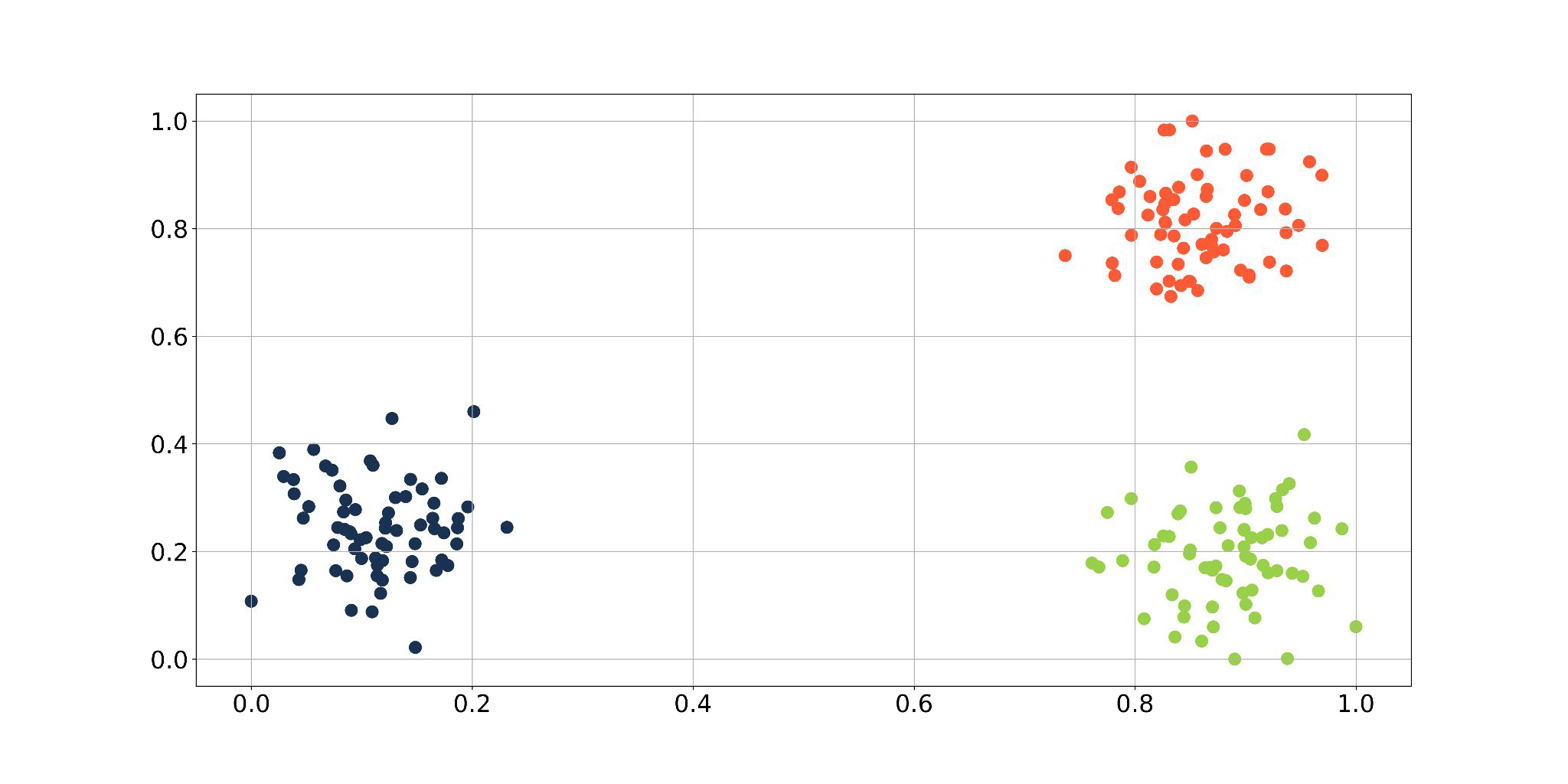
To which category does x belong to?
Blue / Red / Green?
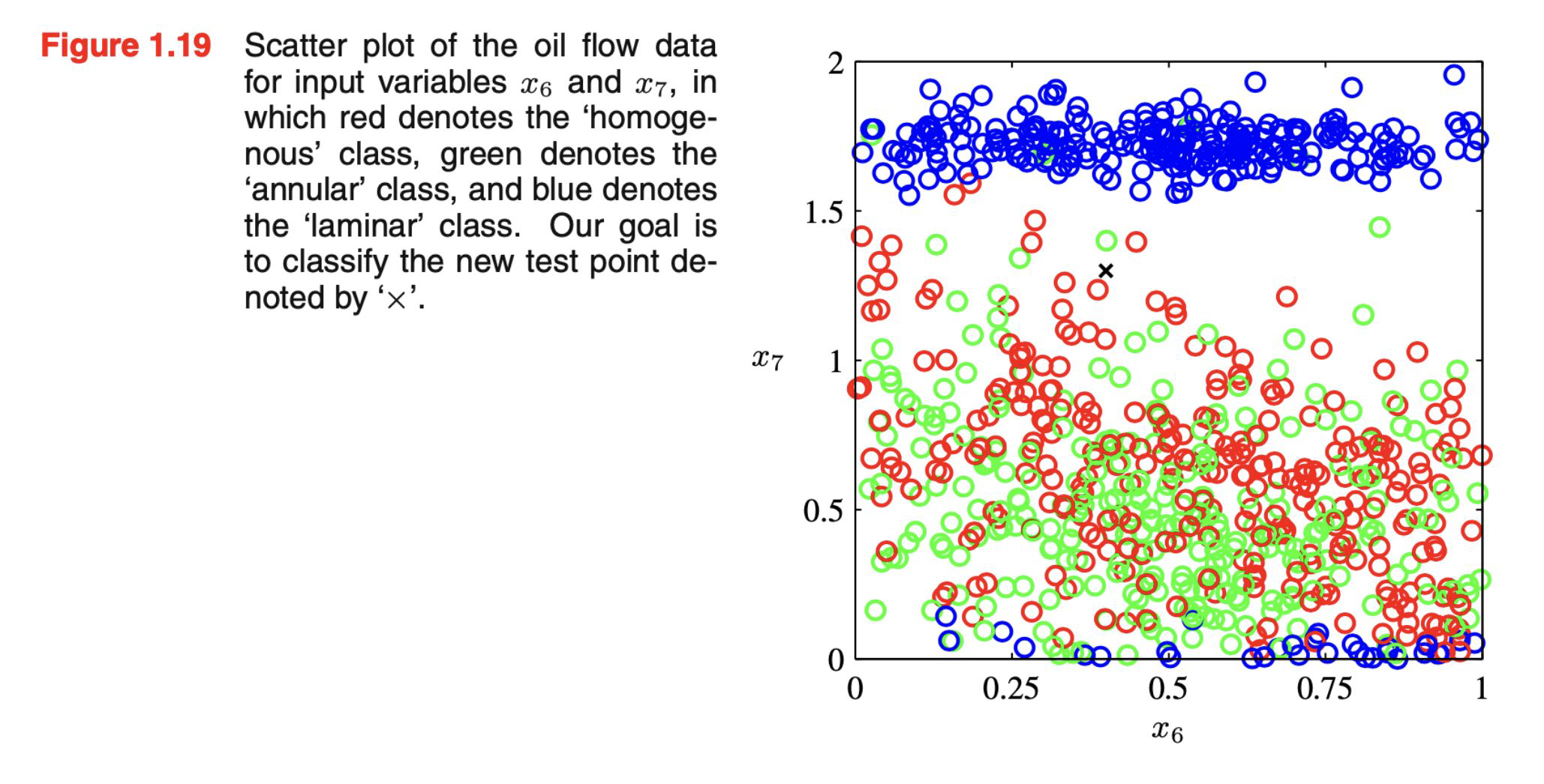
Intuition: The identity of x should be determined more strongly by nearby training points and less so by further away training points
Simple approach: Divide in cells x belongs to the majority class in it’s cell
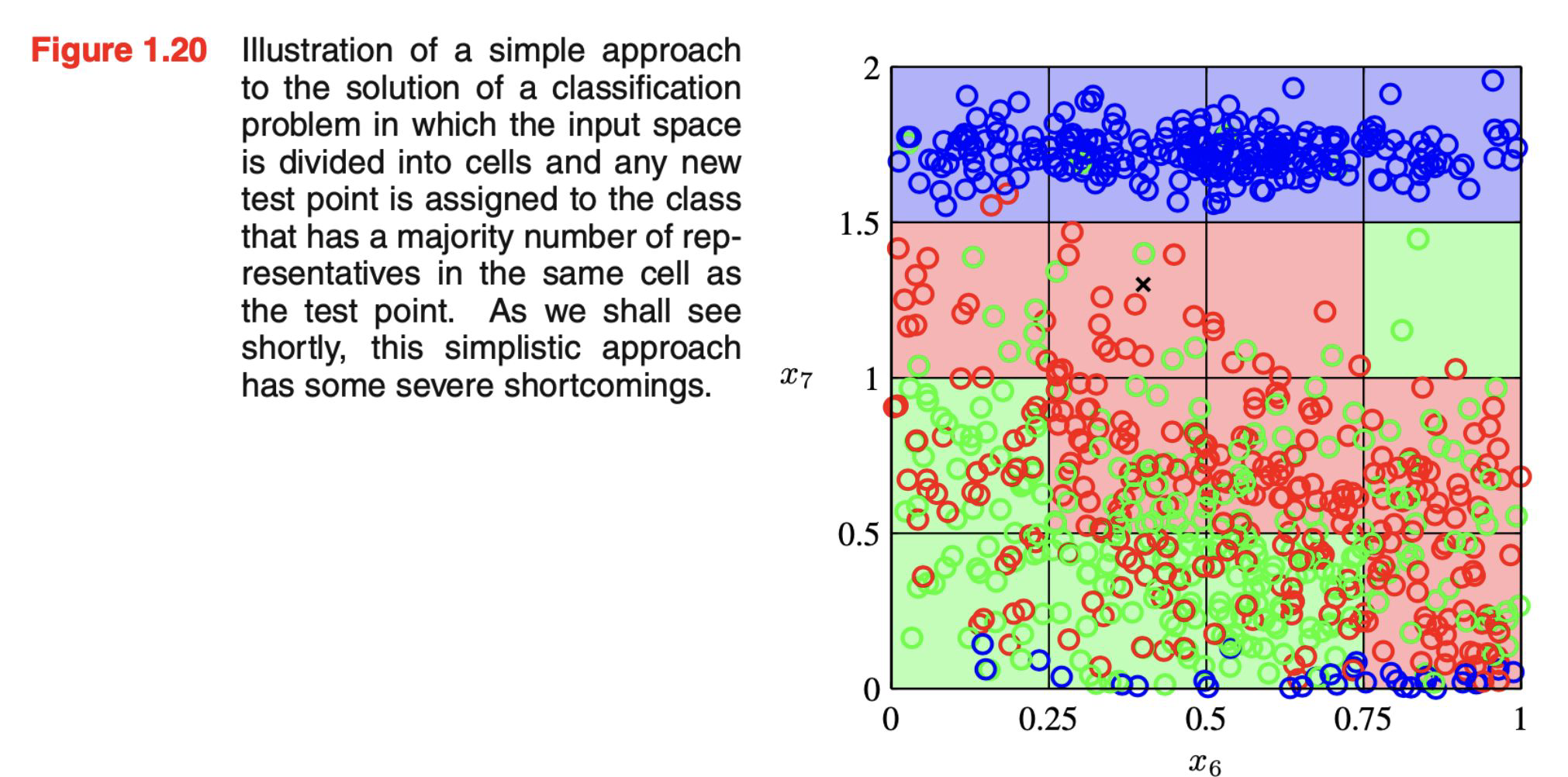
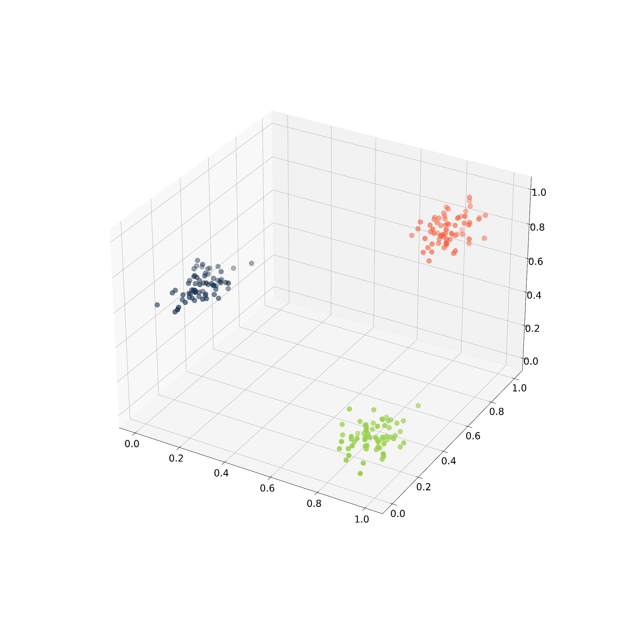
What if we have more dimensions?
The curse of Dimensionality: Intuition#
Do you think in all plots are the same amount of points?
The curse of Dimensionality#
If we divide a region of a space into regular cells, the number of cells grows exponentially with the dimensionality of the space
Why is this a problem?
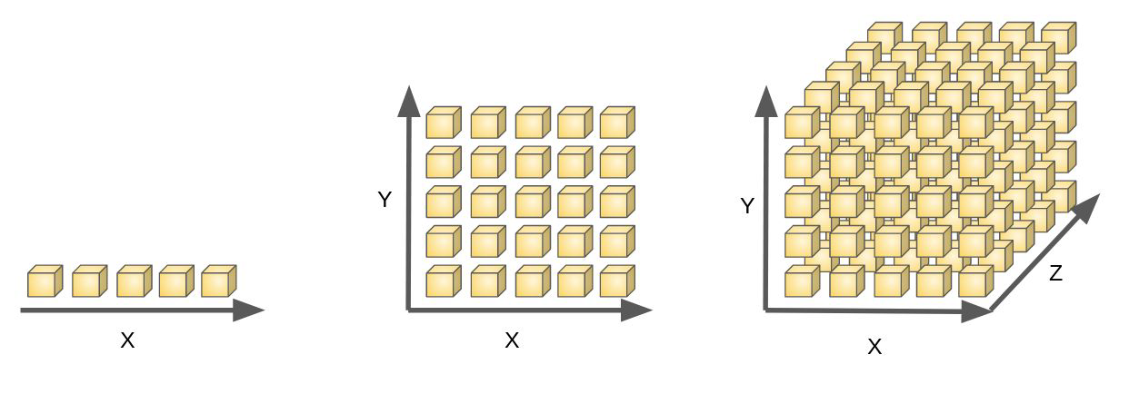
How many data points do we need to cover all the cells?
We would need exponentially large quantity of training data to ensure all cells are filled
Sparse data: when you do not have data covering all cells!
I.e. between radius \(r_\text{i} = 1 - \epsilon \) (where \( \epsilon \) is the thickness of the shell) and \(r_\text{total}\) = 1 ?
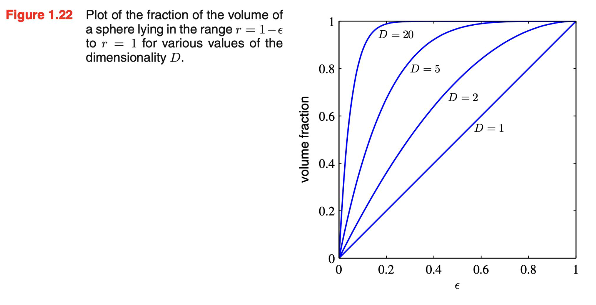

WHYYYYYYY!!????
The curse dimensions..#
we can still apply pattern recognition techniques to high-dimensionality data by exploiting these properties of real data:
may be confined to a region of the space having lower dimensionality, the directions over which important features may vary can be confined
will typically exhibit some smoothness properties and small changes in the input variables will produce small changes in the target variable
use local-interpolation techniques to make predictions for new values
The Manifold Hypothesis#
Real-world high-dimensional data lies on low-dimensional manifolds
manifolds are embedded within the high-dimensional space
manifolds are topological spaces that behave locally like Euclidean spaces
https://deepai.org/machine-learning-glossary-and-terms/manifold-hypothesis
Manifold Hypothesis - Intuition#
“Most real-world high-dimensional datasets lie close to a much lower-dimensional manifold”
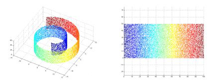
typical example: swiss roll
2D plane, bent and twisted in 3rd dimension
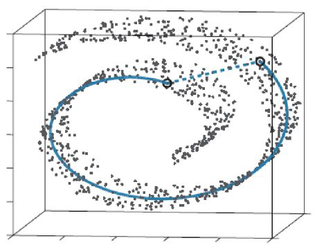
one dimension: line, circle, but not an 8
two dimensions: surface, sphere, plane
purpose is to unroll the swiss roll
the real euclidean distance between the two points is the solid line, not the dotted one
Getting the best point of view = maximizing the line of sight#

Getting the best point of view = maximizing the line of sight#
Advantages#
Speeds up subsequent algorithm
Data compression without substantial loss of information
Helps visualizing patterns
Can improve results through noise reduction (only sometimes)
Disadvantages#
Potential information loss
Computational cost
Transformed features may be hard to interpret
PCA#
Principal Component Analysis#
Goal is to reduce dimensions of feature space while preserving as much information as possible by:
➔ Finding new axis (= principal components) that represents the largest part of variance
principal components must be orthogonal (=independent) to each other
you can have just as many principal components as features
➔ keep only the most informative principal components
Principal Component Analysis#
PCA: combine the numeric predictors into a smaller set of variables, which are weighted linear combinations of the original set
the smaller set of variables, the principal components, explains most of the variability of the full set of variables
the weights reflect the relative contributions of the original variables
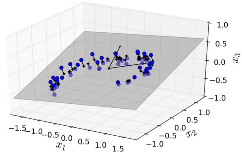
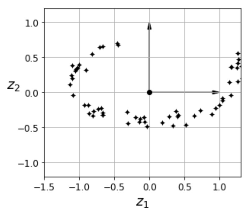
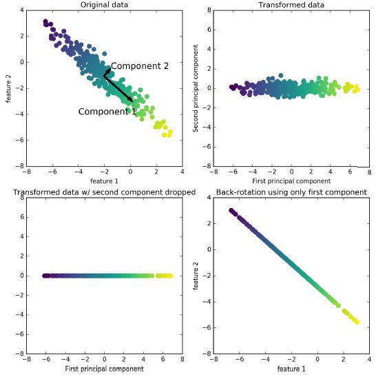
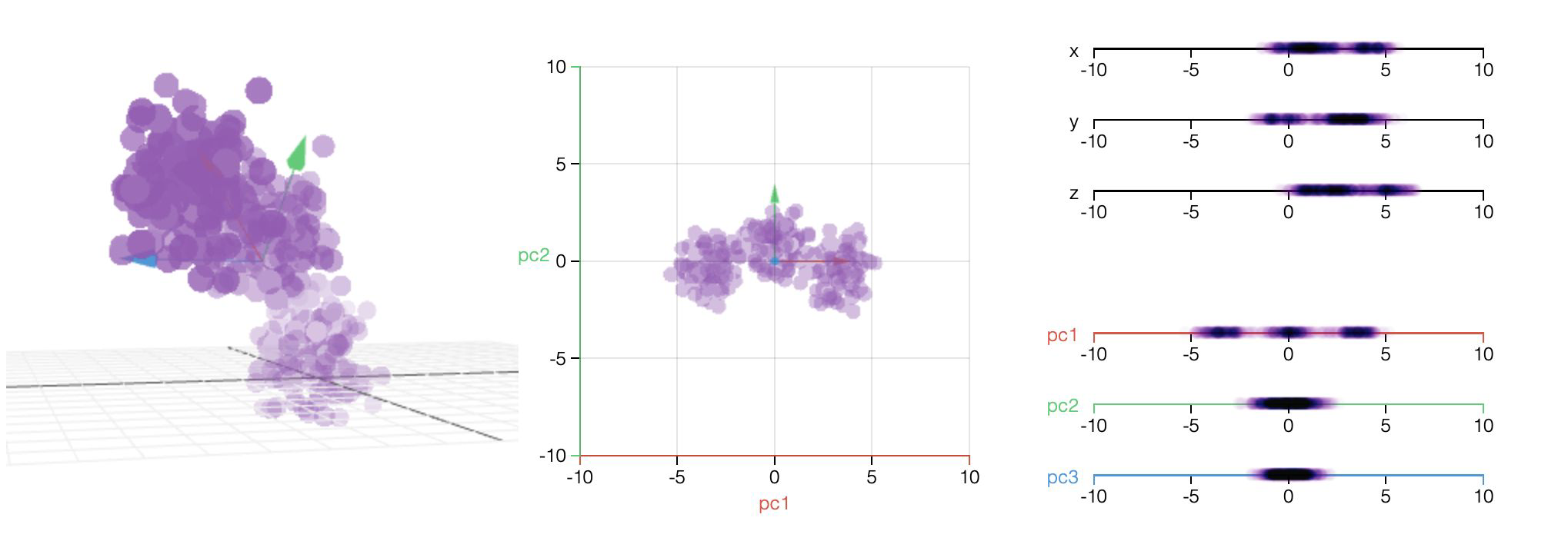
Principal Component Analysis - Projection to lower dimensions#
feature space (3D) reduced to lower dimensional subspace (2D)
the first 2 principal components can be presented as hyperplane
data is projected perpendicularly onto this hyperplane
Principal Component Analysis - Projection to lower dimensions#
Which line would you choose to preserve as much information as possible?
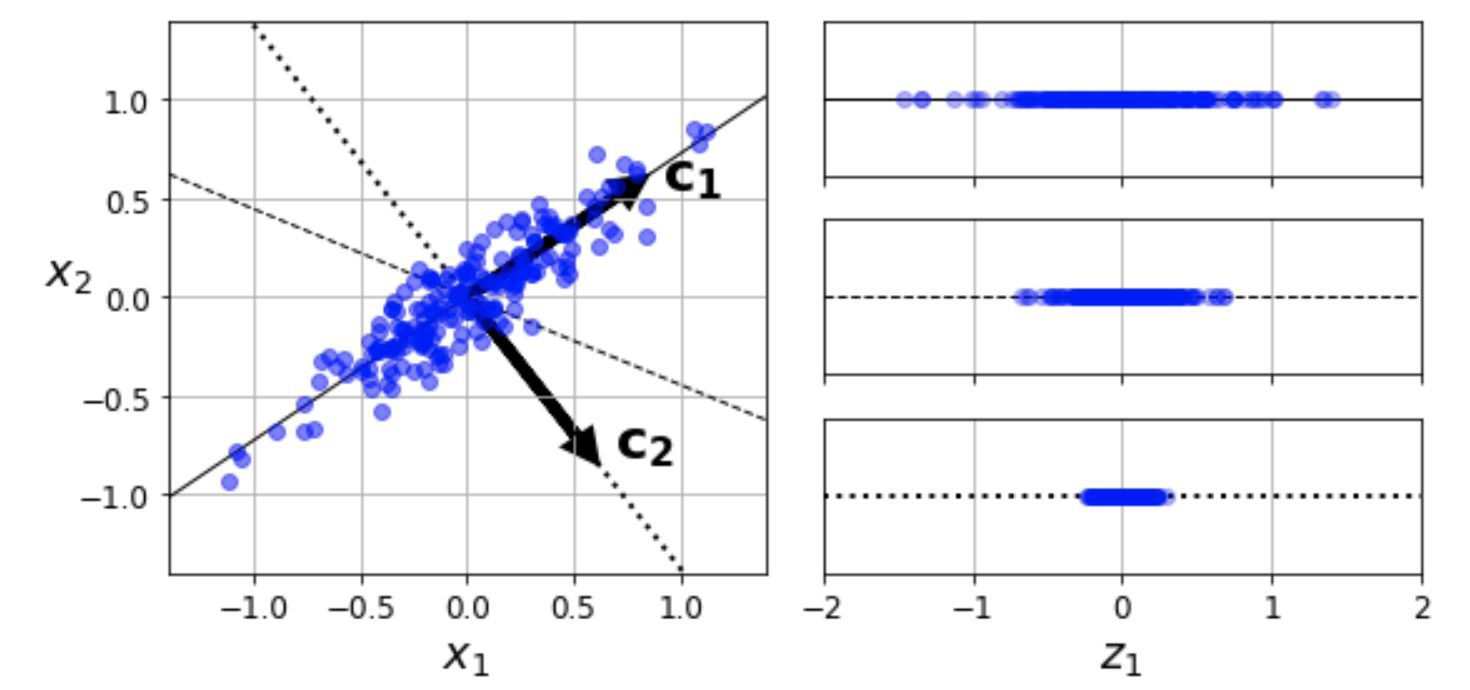
C1 preserves most of the variance
C2 (dotted line) is orthogonal to C1, preserves little variation
The unnamed, dashed line preserves an intermediate amount of variance
Principal Component Analysis - Transformation of Data#
important to transform data for PCA
centered around zero
principal components are combinations of features and can be presented in the original feature space
Principal Component Analysis#

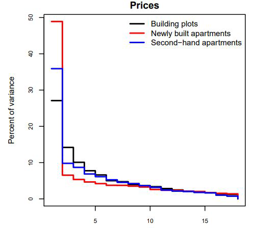
Principal Component Analysis - Explained Variance Ratio#
principal components are found by a standard matrix factorization technique (Singular Value Decomposition (SVD))
after identifying all PC, reduce the dimensionality of the dataset by keeping only the first d PC
→ look at the explained variance ratio of the PCs to decide how many d Dimensions to keep
→ take as many d PC that a sufficiently large portion of the variance is explained (eg 95%)
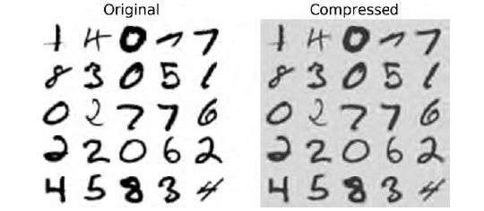
Principal Component Analysis for Compression#
Original Data (left picture)
784 features
PCA
preserving 95% of variance
154 PCs
only 20 % of original size!
Inverse Transformation (right picture)
transforms 154 PC back to 784 features
only slight quality loss
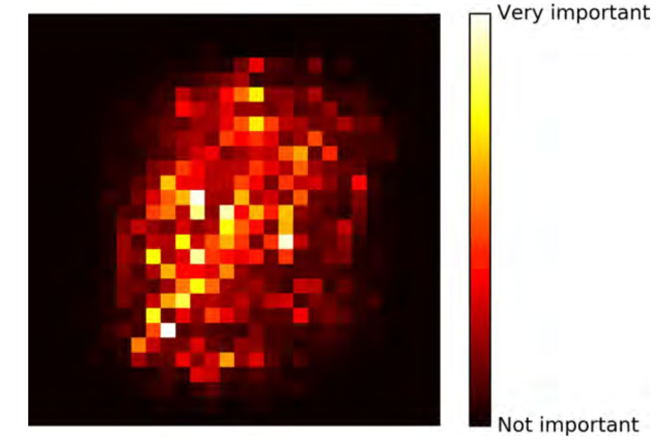
Principal Component Analysis - Eigen Faces#
Eigen Faces: using PCA as a compression algorithm for images
Each image is turned into a vector and PCA is used to get their principal components
Instead of the training images them selves, we use the linear combination of the PCs (here called Eigenfaces due to their apperance) to represent the images.
Before transformation:
47 * 62 pixels (resolution) * 1000 (#Images) = 2.914.000 numbers,
After transformation using 12 Eigen-Faces:
47 * 62 pixels (resolution) * 12 (#Used-Eigen-Faces) + 12 (#Used-Eigen-Faces) * 1000 (#Images) = 46.968 numbers
Each original image can be represented by a linear combination of 12 Eigen Faces. It will appear “blurry” -> but we also only need ~2% of the data to store them
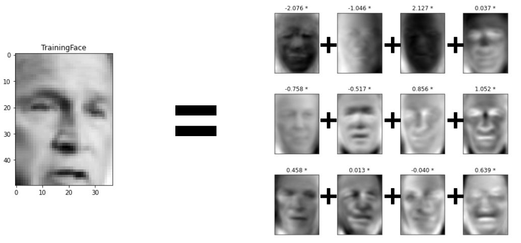
Notes: You can see that each eigen face is focusing on a different aspect of face recognition, e.g. some have black for the eyes, others for the nose bridge, or face shape (identify position). If a few of tehm already focus on the eyes, the other don’t need to because it was already well captured.
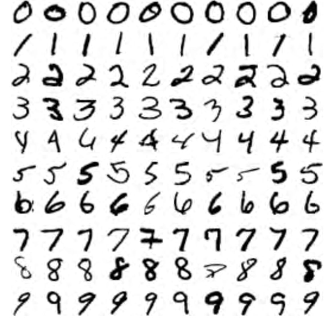
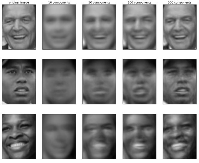
Principal Component Analysis - PC visualization#
with inverse transformation we can see what information is preserved after using different numbers of PCs
original picture: 2914 pixels
Principal Component Analysis - Variants#
Randomized PCA: quick, approximation of first d components
Incremental PCA: for parallelization works with minibatches
Kernel PCA:
Kernel trick
complex nonlinear projections are possible
Preserves clusters of data after projection
can help to unroll data that lies on a manifold
PCA - Use Cases#
reduces the features space dimensionality.. it gets expensive to compute for more than few thousands of features
discards information from the data, downstream model may be cheaper to train, but less accurate
can be used in anomaly detection of time series
financial modeling - factor analysis
preprocessing step when learning from images -> may speed up the convergence of the algorithm
Other Techniques - linear#
Linear Discriminant Analysis (LDA)
→ classification algorithm
→ finds discriminative axes that keep classes as far apart as possible
Latent Semantic Analysis (LSA)
→ does not center the data before computing the singular value decomposition => can work with sparse matrices efficiently
→ also called truncated SVD
Other Techniques - non linear#
t-Distributed Stochastic Neighbour Embedding (t-SNE) → based on probability distribution calculated with the distances between all points
Uniform manifold approximation and projection (UMAP) → works with kNN (=> k is a hyperparamter also in UMAP) → faster than t-SNE
References#
https://github.com/peteflorence/MachineLearning6.867/blob/master/Bishop/Bishop - Pattern Recognition and Machine Learning.pdf
https://en.wikipedia.org/wiki/Manifold https://www.researchgate.net/publication/2953663_Diagnosing_Network-Wide_Traffic_Anomalies
Feature Engineering for Machine Learning
Dogan (2013) Dogan, Tunca. (2013). Automatic Identification of Evolutionary and Sequence Relationships in Large Scale Protein Data Using Computational and Graph-theoretical Analyses.
A. Geron, ”Hands-on ML with scikit-learn and tensorFlow”, 2017
Kholodilin, Konstantin & Michelsen, Claus & Ulbricht, Dirk. (2018). Speculative price bubbles in urban housing markets: Empirical evidence from Germany. Empirical Economics. 55. 10.1007/s00181-017-1347-x. https://www.diw.de/documents/publikationen/73/diw_01.c.487920.de/dp1417.pdf
Müller, Andreas C., and Sarah Guido. Introduction to machine learning with Python: a guide for data scientists. “ O’Reilly Media, Inc.”, 2017.
https://www.geeksforgeeks.org/ml-face-recognition-using-eigenfaces-pca-algorithm/