Logistic Regression#
Recap!#
Confusion Matrix#
Q1: Which cells show the correct predictions
Q2: Now where do we put… TN TP FN FP?
| Predicted | |||
|---|---|---|---|
| Negatives | Positives | ||
| Actual | Negatives | ||
| Positives | |||
Confusion Matrix#
Q1: Which cells show the correct predictions
Q2: Now where do we put… TN TP FN FP?
| Predicted | |||
|---|---|---|---|
| Negatives | Positives | ||
| Actual | Negatives | TN | FP |
| Positives | FN | TP | |
Classification metrics#
Q3: Which classification metrics do you remember?
Metric |
Value |
|---|---|
Accuracy |
\({\frac{130}{200}}=0.65\) |
Precision |
\({\frac{70}{110}}=0.64\) |
Recall |
\({\frac{70}{100}}=0.7\) |
F1-Score |
\(2\cdot \frac{\text{Precision} \cdot \text{Recall}}{\text{Precision} + \text{Recall}}=\frac{2}{3}\) |
ROC AUC |
|
Q4: What are the values?
| Predicted | |||
|---|---|---|---|
| Negatives | Positives | ||
| Actual | Negatives | 60 | 40 |
| Positives | 30 | 70 | |
Accuracy - Rate of corrrect predictions - (TP+TN) /(TP+TN+FP+FN) = # correct predictions / # all predictions
Precision - How precise does a model predict positives - TP / (TP+FP) = # correct positives / # all positives
Recall/Sensitivity/TPRate - How many % of the patients will be recalled / How sensitive is the model - TP / (TP+FN) = # correct positives / # actual positive
F1-Score - Harmonic mean between Precision and Recall - 2x (P*R) / (P+R)
ROC AUC - area under ROC curve; parameter: threshold
Classification metrics#
Q3: Which classification metrics do you remember?
Metric |
Value |
|---|---|
Accuracy |
\({\frac{130}{200}}=0.65\) |
Precision |
\({\frac{70}{110}}=0.64\) |
Recall |
\({\frac{70}{100}}=0.7\) |
F1-Score |
\(2\cdot \frac{\text{Precision} \cdot \text{Recall}}{\text{Precision} + \text{Recall}}=\frac{2}{3}\) |
ROC AUC |
|
Q4: What are the values?
| Predicted | |||
|---|---|---|---|
| Negatives | Positives | ||
| Actual | Negatives | 60 | 40 |
| Positives | 30 | 70 | |
ROC Curve#
Q5: What is the threshold?
Q6: When would you change it?
Improving the recall, TP / (TP+FN) = missing no patient, by altering the threshold goes along with:
a worsening (increase) in false alarms, called false positive rate, because there will be more FP.
Logistic Regression#
Classification#
Some examples for classification
Email: spam vs not spam
Tumor classification: malignant vs benign
Bee image: healthy vs not healthy
Sentiment analysis: happy vs sad
Text analysis: toxic vs not toxic
Face recognition: iphone owner or not
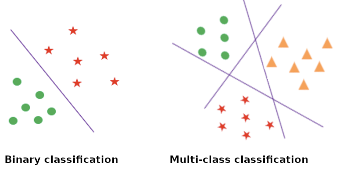
Animal detection: cat vs dog vs monkey vs… (multi class classification)

In (binary)-classification we have two possible classes:
Class 0: the negative class (not spam, malignant, not cat)
Class 1: the positive class (spam, benign, cat)
Why classification?#
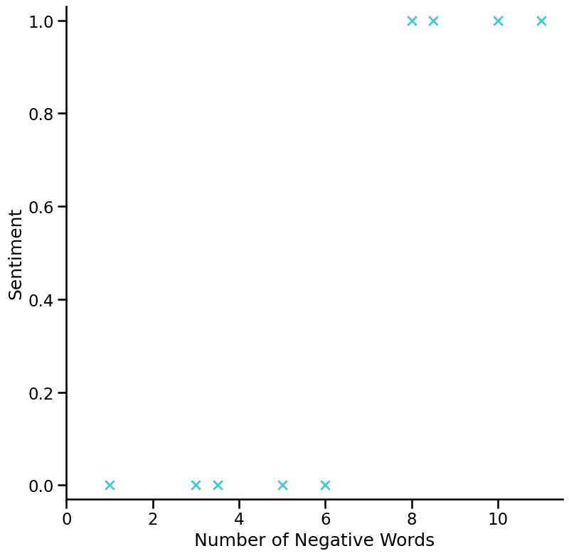
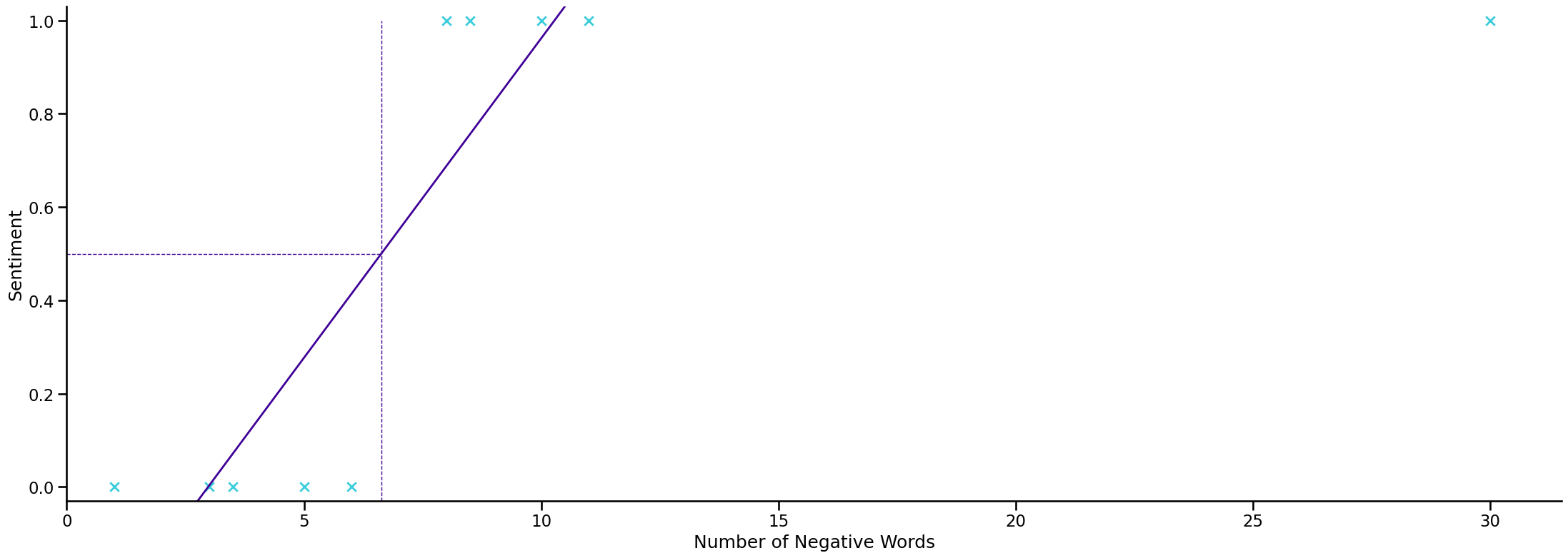
Why do we need another (classification) algorithm if we have linear regression?
Why classification?#
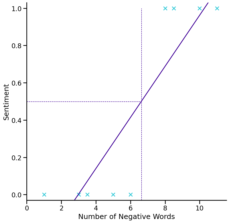
Why classification?#
if \(h_{b}(x)\geq0.5\) then predict “y = 1” (→ sad)
if \(h_{b}(x)<0.5\) then predict “y = 0” (→ not sad)
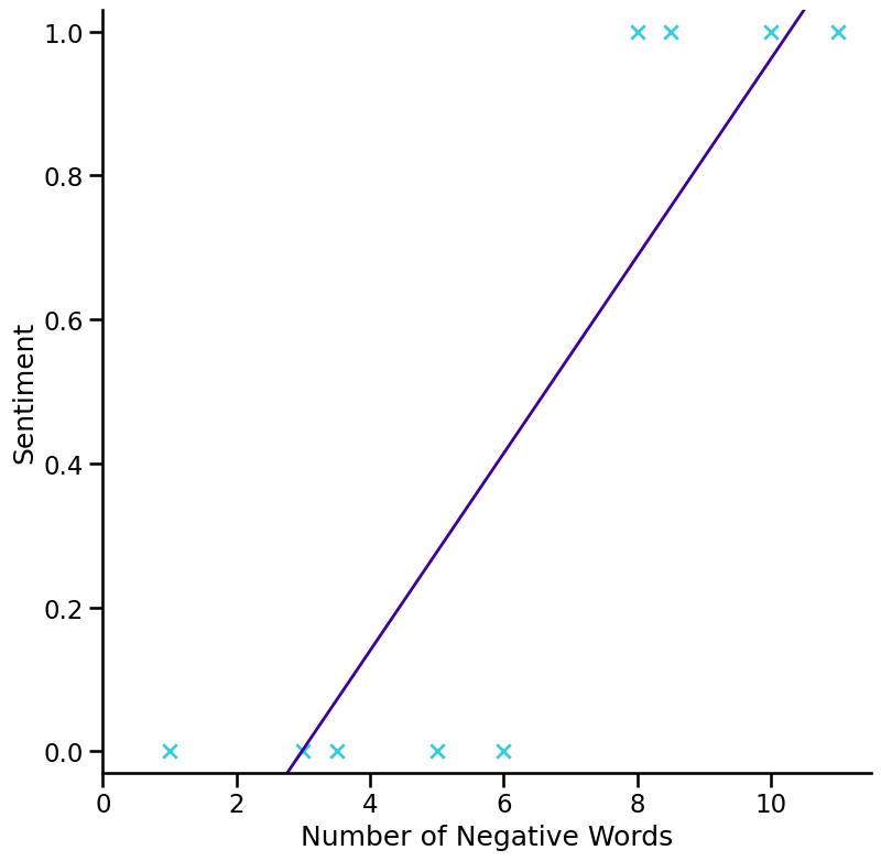
Why classification?#
Why Classification?#
applying linear regression to a classification problem is usually not a great idea
first time we got lucky and we got a hypothesis that worked well for the particular example
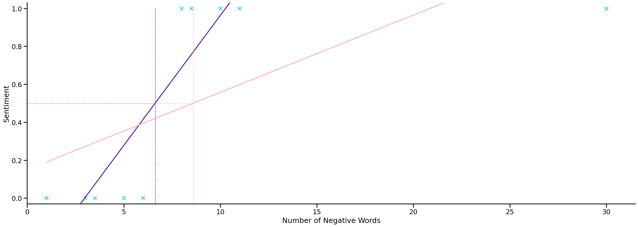
Another problem with classification with linear regression#
y can be 1 or 0 (or any other labels) \(y\in\{0,1\}\)
but the hypothesis \(h_{b}(x)\) can be larger than 1 or smaller than 0 even when all the training data was with 0 and 1
Logistic Regression Model#
Classification hypothesis:
Linear regression hypothesis:
Logistic regression hypothesis:
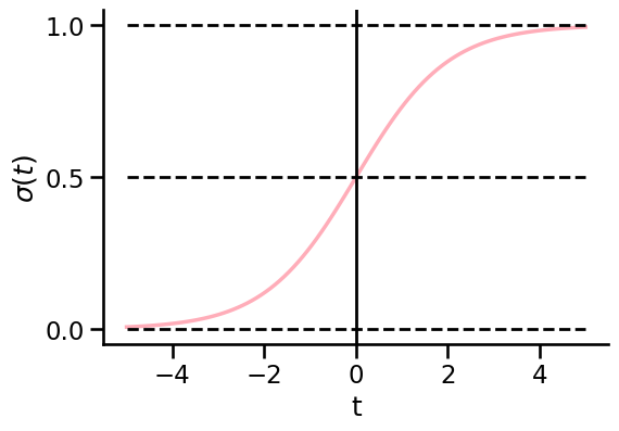
Sigmoid function aka. logistic function:
The Logistic function#
Lets discuss some properties of the sigmoid function:
Sigmoid function makes values fit into (0,1)
The sigmoid asymptotes to 0 when t goes to minus infinity
The sigmoid asymptotes to 1 when t goes to infinity
All its values lie within (0,1)
From logistic function to logistic regression#
Sigmoid function makes values fit into (0,1)
we then need to pick the parameters b
t is equivalent to \(b^Tx\)
Explore the sigmoid function#
Please take this code and evaluate the infuence of \(b_0\) and \(b_1\).
import pandas as pd
from matplotlib import pyplot as plt
import numpy as np

# create the sigmoid function
def sigmoid_function(t):
    '''Calculates p for given t'''
    p = 1/(1+np.exp(-t))
    return p

# create the logit function
def logit_function(x, b0, b1):
    '''Caluculates the border'''
    t = b0 + b1*x
    return t

b0 = 0
b1 = 0.2

x = np.arange(-50, 50, 1)
t = logit_function(x, b0, b1)
p = sigmoid_function(t)

plt.plot(x,p, color=c_dark)
plt.vlines(x=-b0/b1,ymin=0, ymax=1,color=c_blue,linestyle='--', linewidth=1.2)
plt.hlines(y=0.5,xmin=-50, xmax=-b0/b1,color=c_light, linestyle='--', linewidth=1.2)
plt.show()
Explore the sigmoid function#
Result
\(p(t(x))\) (the result of the sigmoid function) or in short \(p(x)\) is mainly only 0 or 1 (about)
\(b_0\) shifts the sigmoid function to the left and right
Larger \(b_1\) sharpens the sigmoid function.
Proper fractions of \(b_1\) smoothens the sigmoid function.
Negative \(b_1\) flips the sigmoid function.
Assuming that \(b_0\) and \(b_1\) are known, we can input any \(x\) (a feature of our machine learning problem), and our sigmoid function tells us whether the observation belongs to category 0 or 1.
The only requirement is to customize the model parameters \(b_0\) and \(b_1\) to our needs / input data so that it can be used to discrimitate/binarize/classify any numerical feature \(x\).
Interpretation of the Hypothesis#
\(h_b(x)\) is the probability that y = 1 on input x
Example:
\(h_{b}(x)=0.8\)
The sentence has a 80% probability of being sad. The probability of y=1 given the feature vector x is 80%
Notation:
\(h_{b}(x)=p(y=1\mid x;b)\)
Conditional probability#
The syntax \(p(y=1\mid x;b)\) denotes a so called conditional probability.
The \(p\) is called probability function or just probability.
\(y = 1\) is the event that we are interested in.
The \( | \) is pronounced “given”, which refers to the following parameters …
… \(x; b\) which describe the conditions under which we are considering the probability.
In this example we want to know the probability that y is 1 (that y belongs to class 1) assuming a certain number of negative words \((x)\) and underlying the given weights for \(b\).
What is:
\(p(y=0\mid x;b)\)
Interpretation of the Hypothesis#
This is a classification problem, so y has to be 0 or 1
The Decision Boundary#
Defining the decision boundary / threshold
we could do 0.5 as the threshold (default in sklearn implementation)
If the probability is bigger than or equal to 0.5 it is classified as 1, else as 0.
For what t is the sigmoid greater than 0.5?
The Decision Boundary#
Defining the decision boundary / threshold
we could do 0.5 as the threshold (default in sklearn implementation)
If the probability is bigger than or equal to 0.5 it is classified as 1, else as 0.
When do we predict y = 0?
Classification#
Now classification will be based on probabilities:
0.5 is the threshold
If the probability is bigger than or equal to 0.5 it is classified as 1, else as 0.
Why 0.5? Good question!
The Logistic Function#
Remember: The threshold corresponds to your business problem!
e.g. decrease # missed (potential) patients by decreasing the threshold (drawback: many healthy get paniced)
Hands on. Example time!#
Decision Boundary Example - Let’s use Logistic regression!#
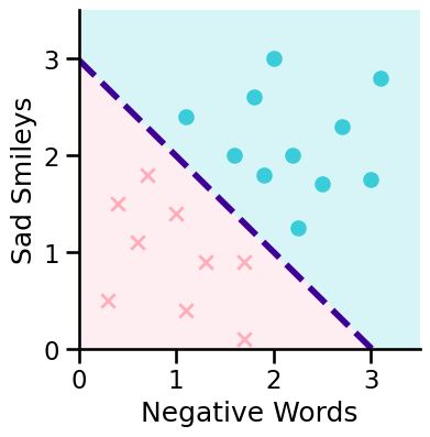
We have some texts to classify as sad (class 1) or happy (class 0)
Our features are:
x1: number of negative words (e.g. “Today was a dull, exhausting and tiring one. 😞”, x1 = 3)
x2: number of sad smileys (e.g. “Today was a dull, exhausting and tiring one. 😞”, x2 = 1)
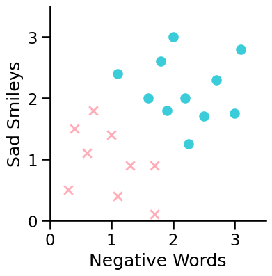
This figure does not show the response this time but two features!
Decision Boundary Example#
\(\hat{p} = \sigma(b_0+ b_1 x_1 +b_2 x_2) = \sigma(b^T x)\)
\(x_0=1\)
\(b^{T} x=\begin{bmatrix}b_0 & b_1 & b_2 \end{bmatrix}\cdot\begin{bmatrix}x_0\\x_1\\x_2 \end{bmatrix}=\,b_{0}\cdot x_{0}\,+\,b_{1}\cdot x_{1}\,+\,b_{2}\cdot\,x_{2}\)
\(x\) is one observation. The index refers to different features:
\(x_0\) belongs to the bias and is 1 (so that \(b_0\) is the intercept).
\(x_1\) and \(x_2\) are the # of neg. words and smileys, resp.
Decision Boundary Example#
\(\hat{p} = \sigma(b_0+ b_1 x_1 +b_2 x_2) = \sigma(b^T x)\)
\(b=\left[\begin{array}{c}{{-3\ }}\\ {{1}}\\ {{1}}\end{array}\right]\)
Decision Boundary Example#
\(\hat{p}= \sigma(b_0+ b_1 x_1 +b_2 x_2) = \sigma(b^T x)\)
\(\hat{p}= \sigma(-3+ x_1 +x_2) = \sigma(b^T x)\)
\(b=\left[\begin{array}{c}{{-3\ }}\\ {{1}}\\ {{1}}\end{array}\right]\)
Decision Boundary Example#
\(\hat{p} = \sigma(-3+ x_1 +x_2) = \sigma(b^T x) = \frac{1}{1+e^{b_0+b_1\cdot x_1 + b_2 \cdot x_2}}\)
We predict class 1 if
\(\hat{p}\geq0.5 \text{ that means } b^T x\geq0\) (the exponent of \(e\))
Decision Boundary Example#
\(\hat{p} = \sigma(-3+ x_1 +x_2) = \sigma(b^T x)\)
We predict “y = 1” when:
\(\hat{p}\geq0.5 \text{ when } b^T x\geq0\)
Decision Boundary Example#
\(\hat{p} = \sigma(-3+ x_1 +x_2) = \sigma(b^T x)\)
We predict “y = 1” when:
\({x_1+x_2\geq3}\)
Decision Boundary Example#
\(\hat{p} = \sigma(-3+ x_1 +x_2) = \sigma(b^T x)\)
We predict “y = 1” when:
\({x_1+x_2\geq3}\)
We predict “y = 0” when:
\({x_1+x_2<3}\)
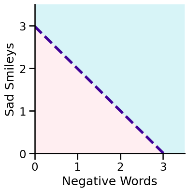
Decision Boundary Example#
We predict “y = 1” when:
\({x_1+x_2\geq3}\)
We predict “y = 0” when:
\({x_1+x_2<3}\)
Decision Boundary:
Decision Boundary#
The decision boundary is a property of the hypothesis and not of the data.
We fit the model to find the parameters b and then we can get the decision boundary based on b.
Spoiler alert: if you use higher order polynomial features you get a non-linear decision boundary.
The Cost Function#
Training set: \(\{(x^1, y^1), (x^2, y^2), ... (x^n, y^n)\}\)
How do we chose the right parameters b?
Fitting the parameter b to the data.
The top numbers are no exponents but refer to the observation number here.
The Cost Function#
For logistic regression the log loss function LLF (also referred to as binary cross entropy) is used:
$\(LLF = -\frac{1}{n}\sum_{i=0}^n\Bigg[ \Bigg(y_i \ln(\hat{p}(x_i))\Bigg) + \Bigg((1-y_i) \ln(1-\hat{p}(x_i))\Bigg)\Bigg]\quad\)$
with \(n\) being the number of observations,
\(y_i\) being the real observations (0 or 1)
and \(\hat{p}(x_i)\) being the predictions, between 0 and 1
\(y_i\) (real value) |
\(\hat{p}(x_i)\) (prediction) |
val in [] |
|---|---|---|
0 |
\( \sim 0\) |
\( \sim 0\) |
0 |
\(\neq 0\) |
large |
1 |
\( \sim 1\) |
\( \sim 0\) |
1 |
\(\neq 1\) |
large |
→ The further the prediction is from the real value, the larger the LLF
vice versa: The smaller the loss, the better the prediction.
The Cost Function#
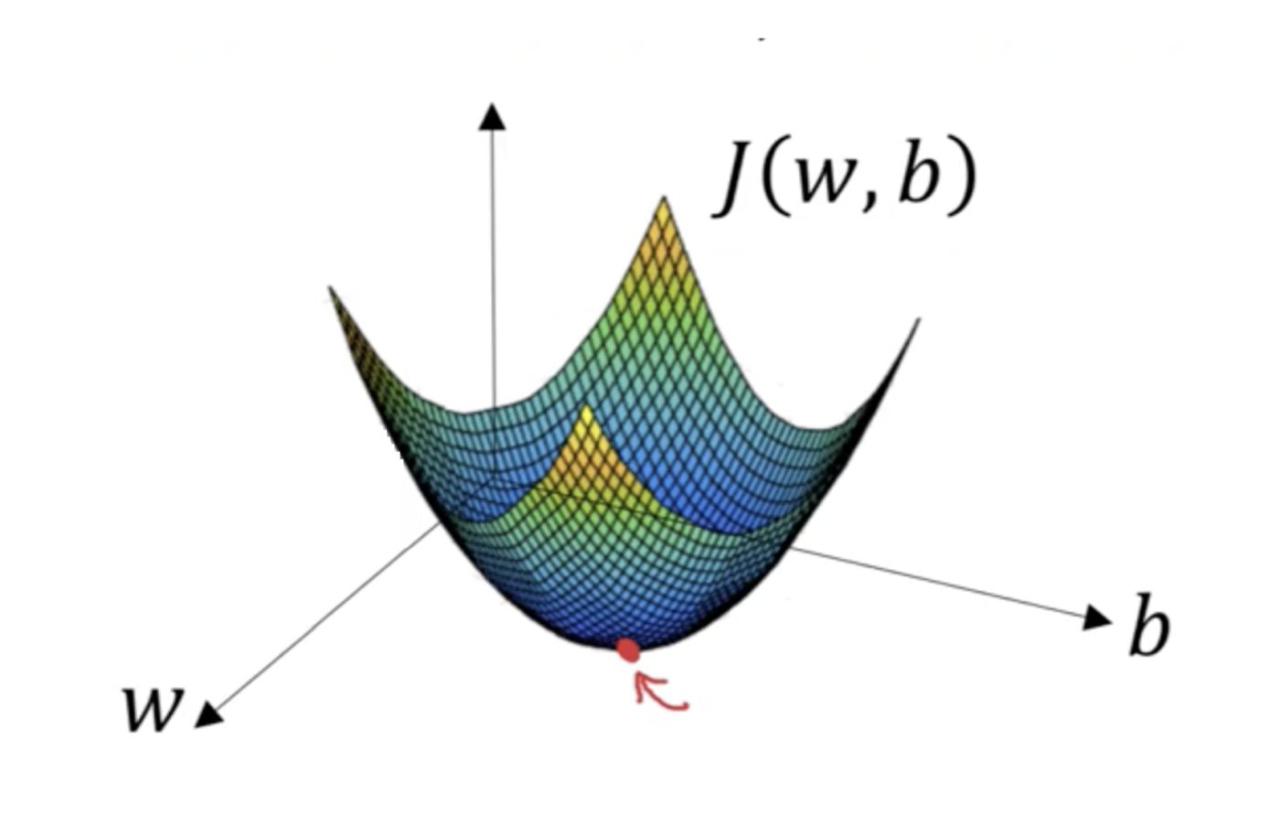
Why don’t we use the cost function we know from linear regression?
This would lead to a non-convex function which is hard to optimize. (Remember: Gradient Descent)
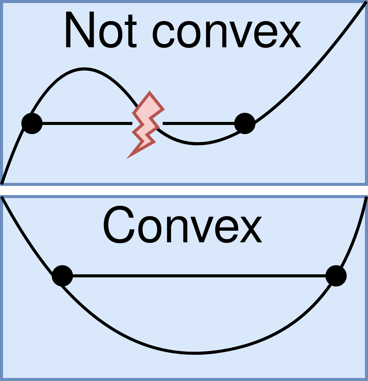
The Cost Function#
The linear regression cost function (remember OLS).
Logistic regression hypothesis:
This would though lead to a non-convex function which is hard to optimize. The usual way to optimize is to find the global minimum.
The Cost Function#
Logistic regression hypothesis:
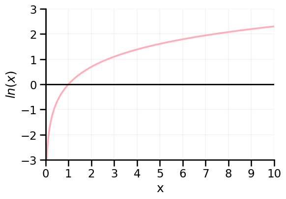
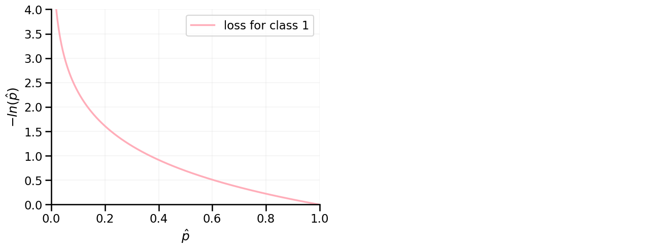
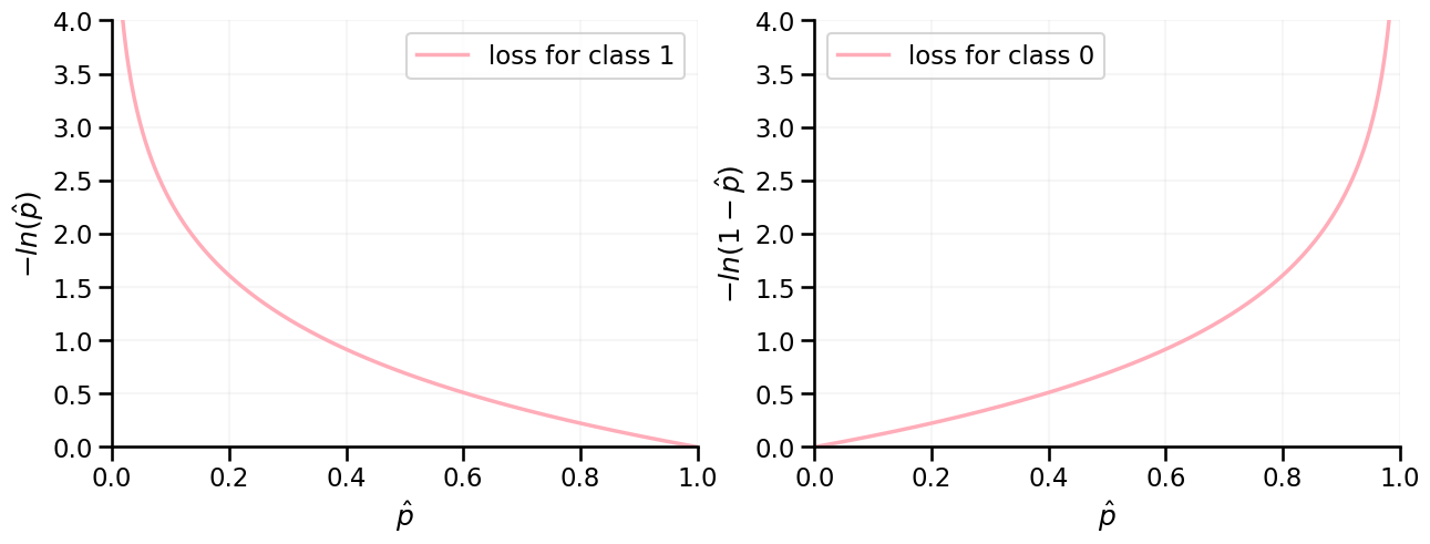
Loss based on logs of probabilities#
For instances belonging to class 1 → Loss is the negative log of \(\hat{p}(y=1)\)
→ Probability is close to zero? Loss is high!

→ Probability is close to one? Loss is low!
For (correct) probabilities of 0 / 1, the loss would be zero.
Loss based on logs of probabilities#
For instances belonging to class 0 → Loss is the negative log of \(1-\hat{p}(y=1)\)
→ Probability is close to zero? Loss is low!

→ Probability is close to one? Loss is high!
For (correct) probabilities of 0 / 1, the loss would be zero.
Now, just add it all up#
Because y is always 0 or 1 we can write this:
Now, just add it all up#
Because y is always 0 or 1 we can write this:
This loss function (binary cross-entropy) can be directly obtained from MLE (maximum likelihood estimation)
From loss to cost#
Now, let’s average the Loss function over all observations:
Now we can fit our parameters b to our data:
Find b that minimizes the cost function J(b).
To minimize the cost function we use gradient descent!
Minimizing J - find \(b\)#
There is no closed form solution as the Normal Equation (\(b = (X^TX)^{-1}X^Ty\)) for linear regression.
So instead we get the partial derivatives and start the gradient descent!
</div>
<div class="images_30">
Conclusion#
Training the model ~ finding b that minimizes J ~ finding the shape of the decision boundary.
Changing the classification threshold from 0.5 (default) ~ changing the position of the decision boundary (but not the shape).
Multi class problems#
How can more than two different classes be predicted?
This is often done using OvR (one versus rest).
If there are 3 classes, 3 classification runs were performed:
class 0 vs. classes 1 \(\cup\) 2
class 1 vs. classes 0 \(\cup\) 2
class 2 vs. classes 0 \(\cup\) 1
The class with the highest probability is used for final prediction.