Time Series Analysis#
Agenda#
Introduction
ARIMA-Family
TSA Decomposition
Smoothing
Fancy models
What is a Time Series?#
A series of data points over time
Q: Examples

What is a Time Series?#
A series of data points over time
Q: Which is a time series?
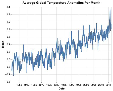
average monthly temperatures 1980-2021
average sales of sneakers in January 2021
the latest song by Billie Eilish
Some temperature data#
Date |
Mean |
Year |
Month |
|
|---|---|---|---|---|
794 |
1950-10-06 |
-0.20 |
1950 |
10 |
795 |
1950-09-06 |
-0.10 |
1950 |
9 |
796 |
1950-08-06 |
-0.18 |
1950 |
8 |
797 |
1950-07-06 |
-0.09 |
1950 |
7 |
798 |
1950-06-06 |
-0.06 |
1950 |
6 |
799 |
1950-05-06 |
-0.12 |
1950 |
5 |
800 |
1950-04-06 |
-0.21 |
1950 |
4 |
801 |
1950-03-06 |
-0.06 |
1950 |
3 |
802 |
1950-02-06 |
-0.26 |
1950 |
2 |
803 |
1950-01-06 |
-0.30 |
1950 |
1 |
What is special in time series data?#
It can (needs to) be ordered by time
Actual values depend on historical ones
Dependent variable stands on both sides of the equation
Even the error terms can depend on historical values
85% of today’s temperature can be explained by yesterdays!
What is special in time series data?#
It can (needs to) be ordered by time
Actual values depend on historical ones
Dependent variable stands on both sides of the equation
Even the error terms can depend on historical values
Distributions can change over time
non-stationarity (hard)
Predicting the future… mhm#
We have no way of knowing (or seriously guessing for that matter) the next outcome of a random experiment. But there is some stuff that we can do!
Pry all information from our data that is not random, and make forecasts from that. Ideally, the remaining error should only be white noise.
Job of a good TSA
split the systematic and the unsystematic
identify both
forecast the systematic
define the unsystematic
EDA for Timeseries#
Visualization#
Visualization is the most important (EDA) tool
Gives a good impression of stylized facts
Trends and/or cycles?
Are there missing values? Are there patterns in missing values?
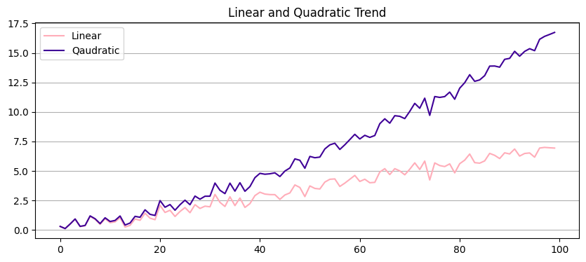
Trends#
Trends are long-term information
Long-term tendency of values
Can show any non-cyclical behavior (linear, quadratic)
Difficulty from trends
Visualizing short-/mid-term is masked)
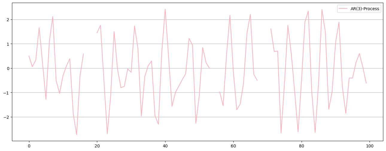
Modelling the values at different time intervals have different levels
Distribution is time-dependent
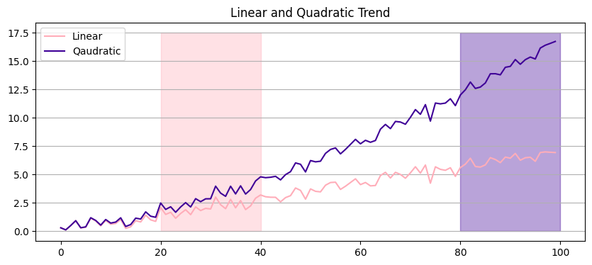
Values in x=[20-40] have very different values from values in x=[80-100]
Eliminating trends#
How to eliminate trends?
Model + subtract trends
linear \( m_t = \alpha_0 + \alpha_1 t \)
quadratic \( m_t = \alpha_0 + \alpha_1 t + \alpha_2 t^2 \)
Differencing \(\Delta y_t = y_t - y_{t-1}\)
(High-Pass Filtering: e.g. Hodrick-Prescott)
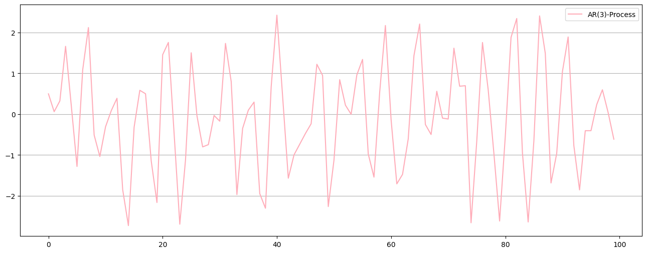
Time series before and after eliminating the trend: afterwards short-/mid-term patterns are clearer
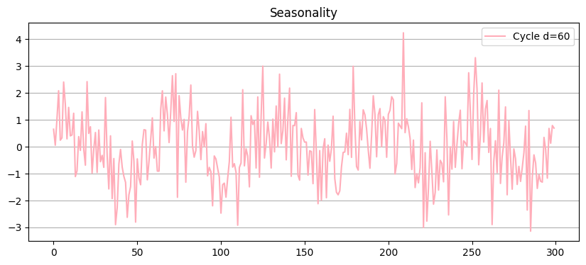
Cycles - and on and on it goes#
Seasonal patterns (cycles) are mid-/short-term information
Recurring value levels
Typical example: sales during the year
Can show any cyclical behavior(e.g. Trigonometric)
Problematic in time series modeling
Values in different areas of the cycle are significantly different
Different distribution - non-stationary
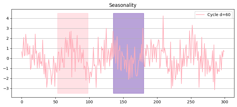
Value distributions look different at different time ranges
Eliminating cycles#
Cycles often contain process-intrinsic information
Eliminate cycles with
Model + subtract trends
Time differencing: \(\Delta y_t = y_t - y_{t-4}\)
Low-pass filtering
Fourier series:
\( s_t = \beta_0 + \sum_{j=1}^{k} (\beta_j \sin(\lambda_j t) + \kappa_j \cos(\lambda_j t))\text{, }\lambda_j = \frac{2\pi}{d_j} \)
Time series before and after removing trend and seasonal patterns… what a beauty
Recap:#
We talked about timeseries data:
Data were the sequence plays a crucial role
Typically: data with a fixed interval without missing values
We talked about visual EDA:
Trends (Where are they coming from? how to deal with that?)
Cycles (Many examples, what to do with that?)
Triggerwarning#
Timeseries?#
DON’T PANIC#
Common Tools in TSA#
Data#
Imputation#
filling (backfilll,forwardfill,mean)
interpolate / filtering
Resampling
Predicting
Train - Test - Split#
Q: How would you split a Timeseries?
Train - Test - Split#
Q: How would you split a Timeseries?
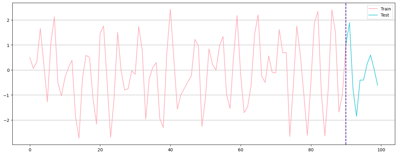
train,test = data[:-10],data[-10:]
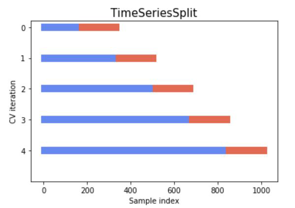
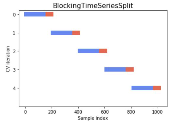
Crossvalidation#
Stationarity#
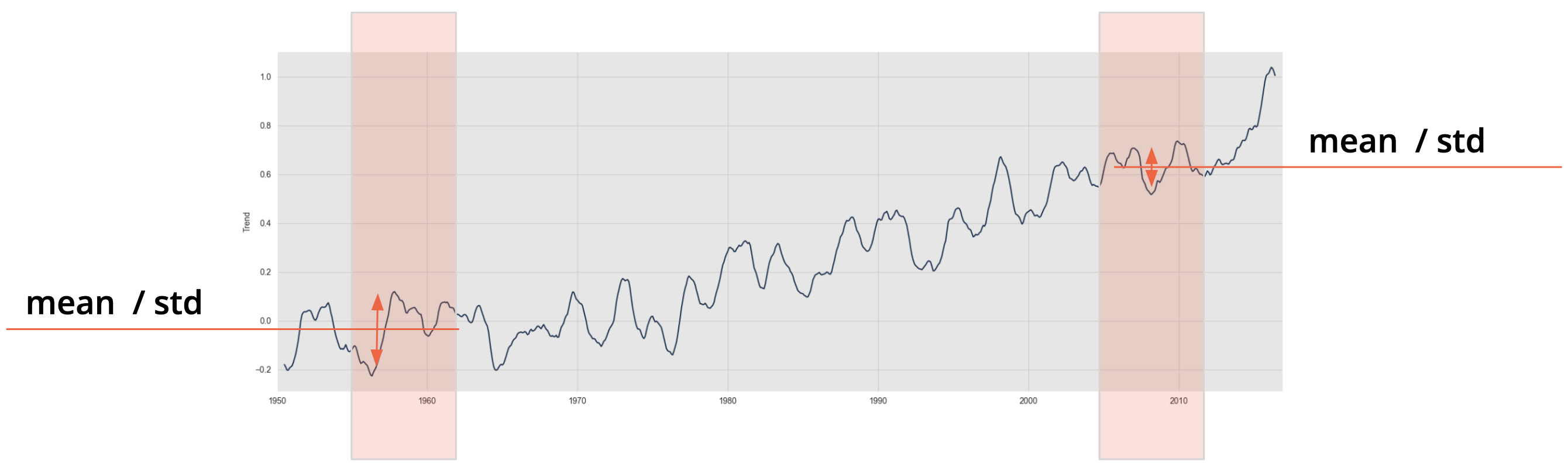
What does it mean for a TS to be stationary?#
Having a constant mean and covariance function across the time series - in short: constant moments
A time series needs to be stationary in order to make good predictions
How do we know?
ADF test - Null Hypothesis: Not Stationary
KPSS test - Null Hypothesis: Stationary
We can also look at the autocorrelation function ACF
Rolling Mean#
Carefull: This rolling mean is actually an AR(p) process, not a MA(q)
Exponential Smoothing Methods#
Modelling Time Series#
The oldschool stuff - Decomposition#
What makes a time series?#
A simple additive decomposed model
\(m_t\) is the trend
\(s_t\) is the seasonality
\(e_t\) is the error or random noise
Trend -> increase or decrease of the values in the series
Seasonality -> the repeating short term cycles in the series
Random noise -> random variation in the series though there might also be some autocorrelations that can be discovered?!
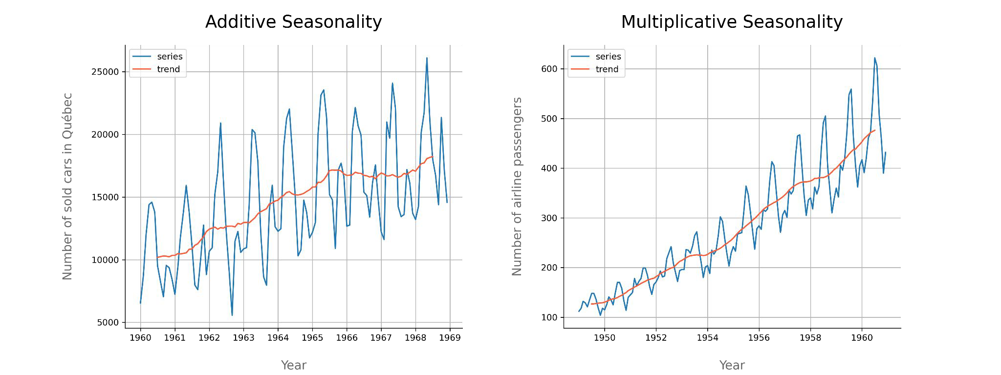
Additive vs Multiplicative#


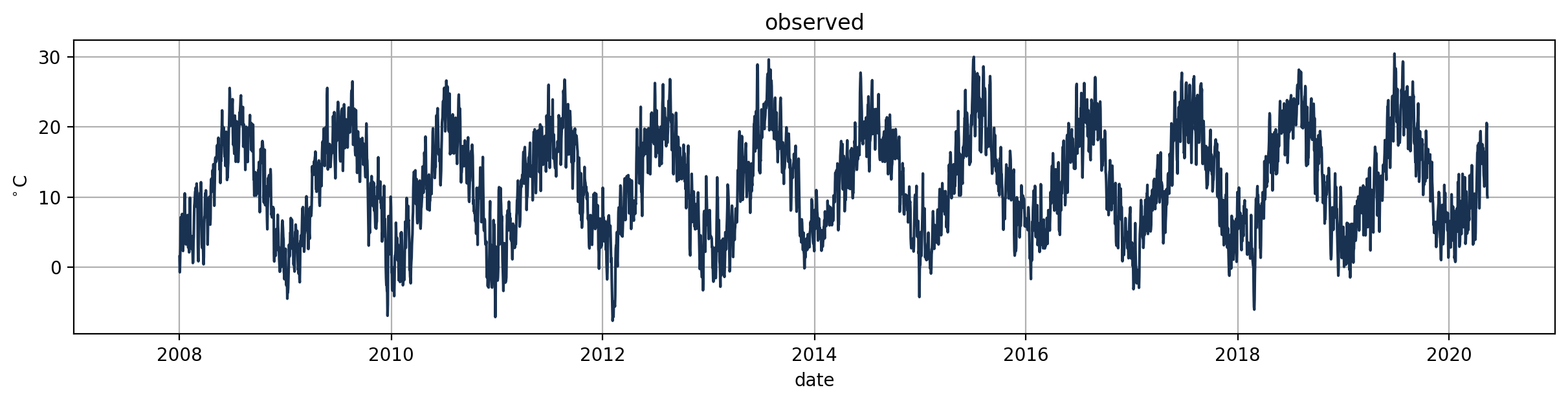
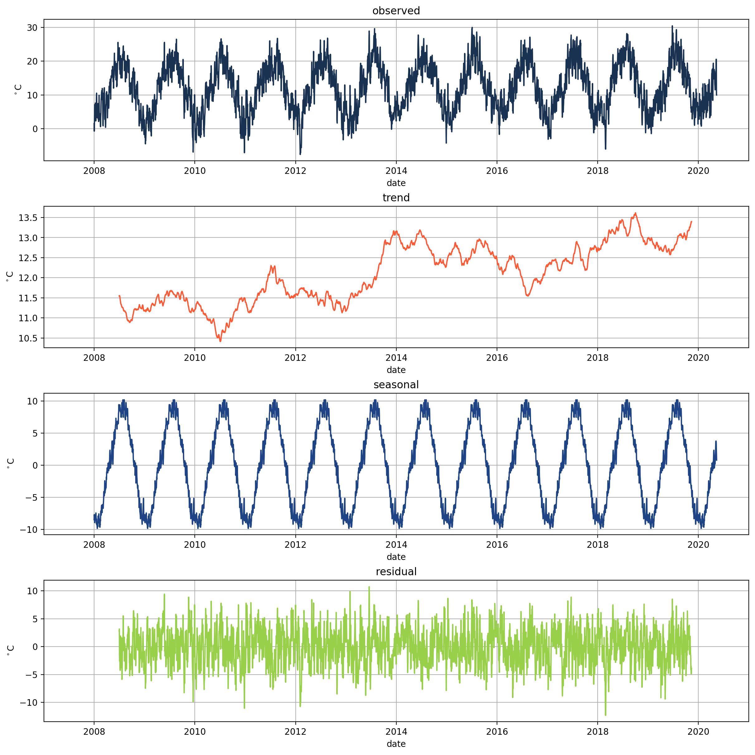
Components of TS#
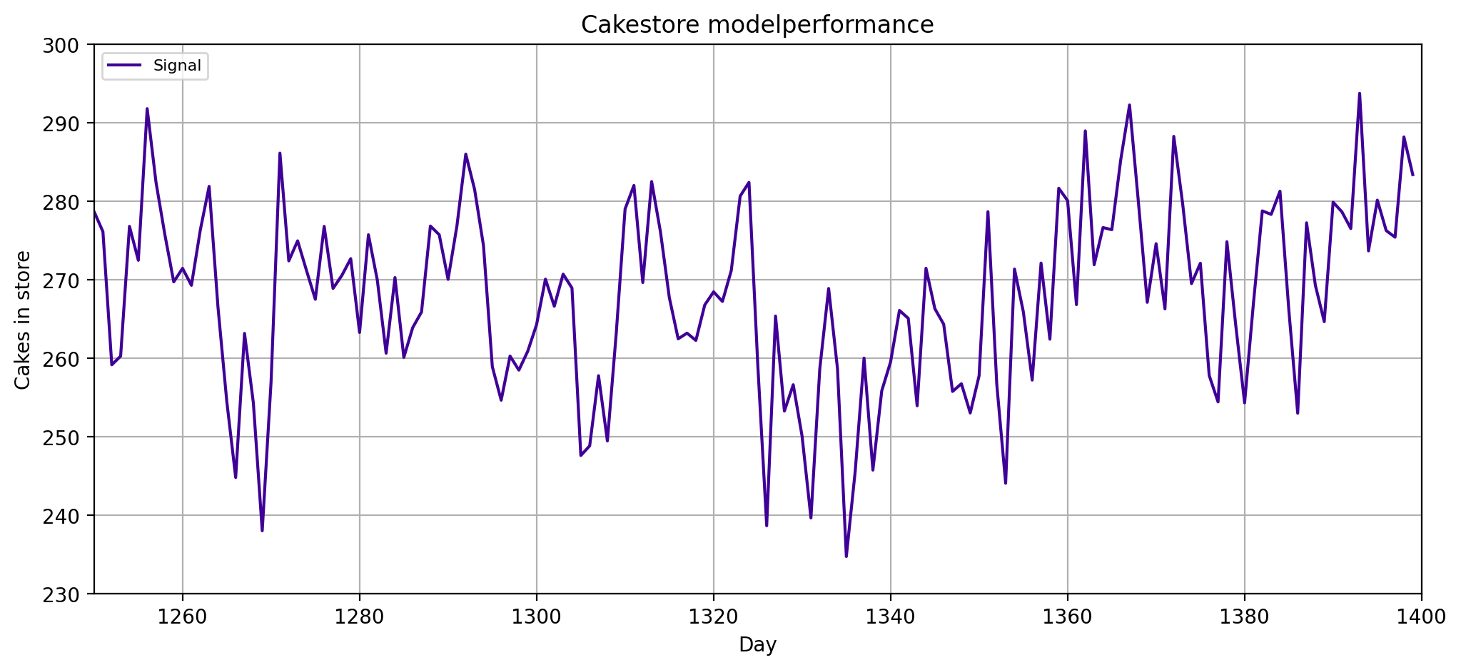
Signal#
Temperature measurements in Basel
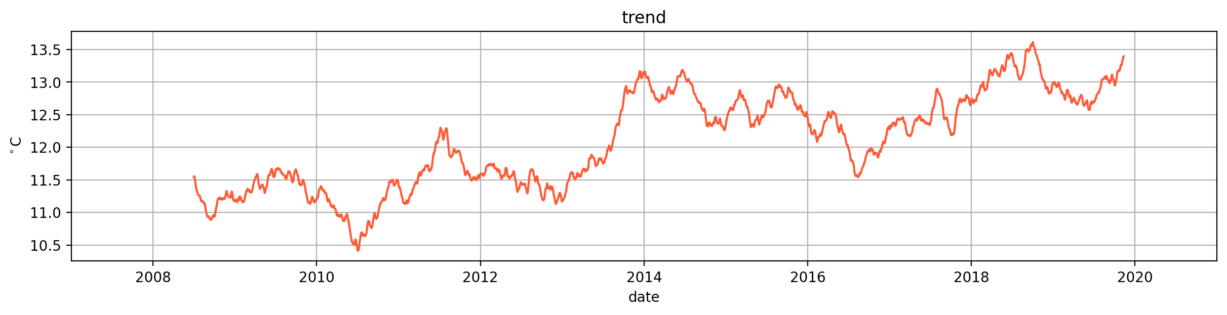
Trend#
What does the trend look like for the temperatures?
(strong) upward trend
temperature is gradually rising
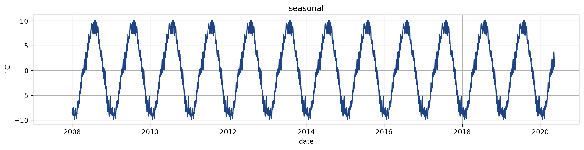
Seasonality#
What does the seasonality look like for the temperatures?
We see a strong seasonality for summer and winter
in business cycles we have the problem of very long cycles - so very long persistence
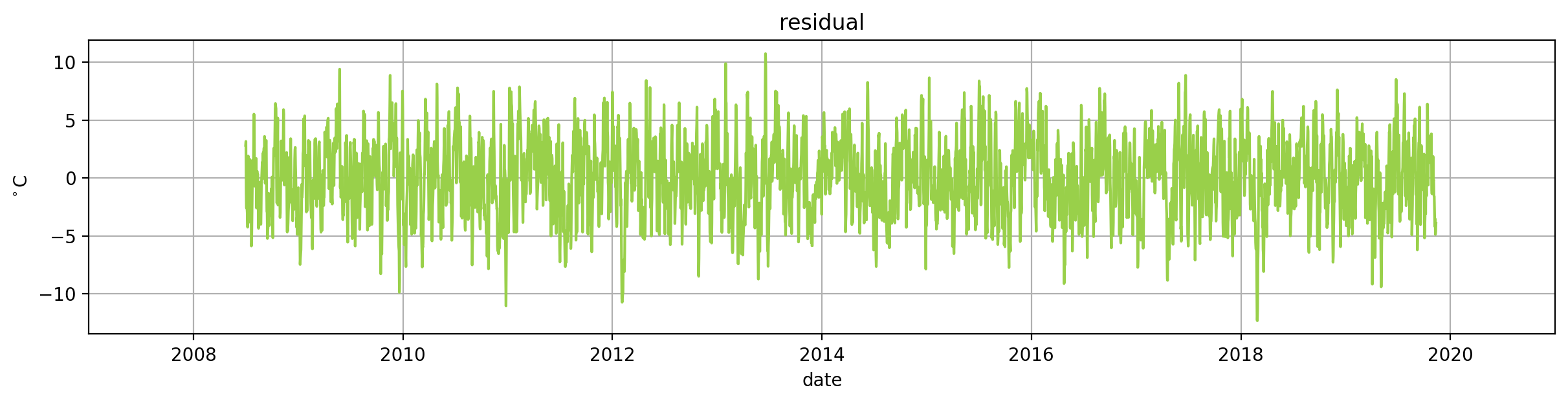
Residuals#
We want residuals to look random
it is random looking
it shows the variation in the series
unexplained variance happening due to chance
Components of TS#
The oldschool stuff - ARMA#
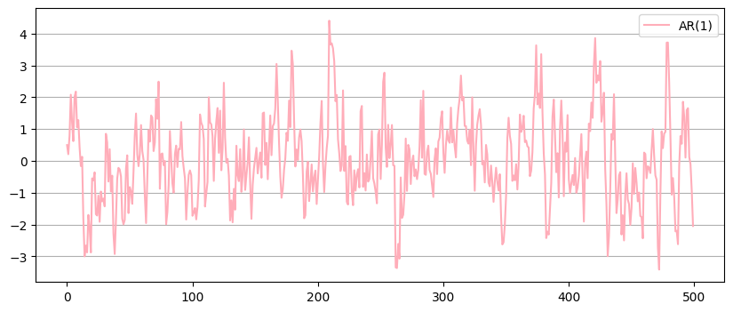
Data Generating ARMA process example#
Store
Current stock of cake \(\hspace{0.5cm}X_t\)
Production
About 100 cakes are produced every day \(\hspace{2cm}\varepsilon_t\)
(normally distributed)
Thieves!
15% of the cakes from stock
are eaten by Larissa
Sales
40% of the production are picked up
the next day
20% of the production are picked up
the day after
\(X_t = \underbrace{0.85 X_{t-1}}_{\text{AR(1)}} \underbrace{- 0.2\varepsilon_{t-2} - 0.4\varepsilon_{t-1}}_{\text{MA(2)}} + \varepsilon_t\)
Data Generating ARMA process example#
\(X_t = \underbrace{0.85 X_{t-1}}_{\text{AR(1)}} \underbrace{- 0.2\varepsilon_{t-2} - 0.4\varepsilon_{t-1}}_{\text{MA(2)}} + \varepsilon_t\)
Data Generating ARMA process example#
print_rmse()
Train RMSE of predict_mean: 11.32
Train RMSE of predict_ARMA: 9.88
Test RMSE of predict_mean: 12.58
Test RMSE of predict_ARMA: 12.27
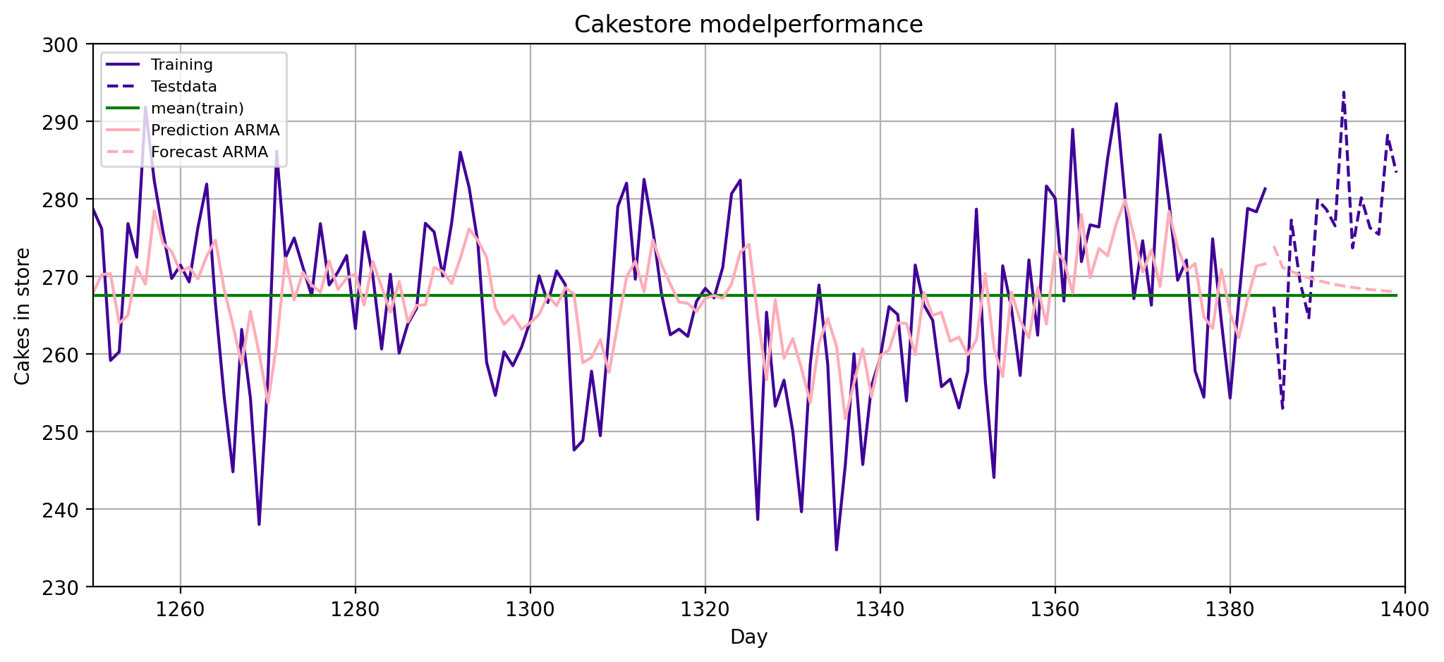
\(X_t = \underbrace{0.85 X_{t-1}}_{\text{AR(1)}} \underbrace{- 0.2\varepsilon_{t-2} - 0.4\varepsilon_{t-1}}_{\text{MA(2)}} + \varepsilon_t\)
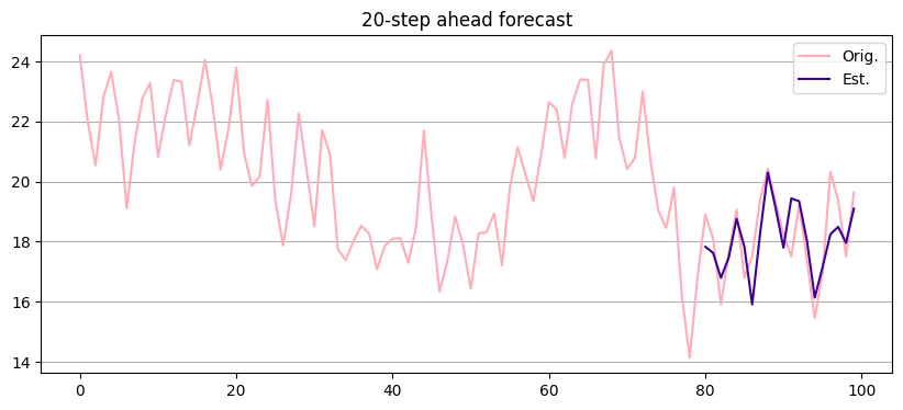
Forecasting with ARMA#
Step 1: Estimate ARMA model
get parameters
Step 2: Use parameters to forecast
calculate innovations recursively
compute forecasts with observations and innovations
software-implemented (statsmodels)
Other models from ARMA class#
ARMAX
Adding exogeneous variables to the model
ARIMA
Adding an integrated part for non-stationarity (in the mean)
SARIMA
Adding a further seasonal part to the model
ARFIMA
Models with long memory
VAR
Multivariate (vector) autoregressive models
Time-Varying coefficients
The “normal” stuff#
With a little trick you can also use many of the models we have used so far (often XGboost is working very well)
| y | |
|---|---|
| 0 | 0.496714 |
| 1 | 0.060421 |
| 2 | 0.324157 |
| 3 | 1.660069 |
| 4 | 0.209006 |
| 5 | -1.280167 |
| 6 | 1.086848 |
| 7 | 2.119192 |
| 8 | -0.510608 |
| 9 | -1.036433 |
| y | y_t1 | y_t2 | y_t3 | y_t4 | y_t5 | y_t6 | |
|---|---|---|---|---|---|---|---|
| 0 | 0.496714 | NaN | NaN | NaN | NaN | NaN | NaN |
| 1 | 0.060421 | 0.496714 | NaN | NaN | NaN | NaN | NaN |
| 2 | 0.324157 | 0.060421 | 0.496714 | NaN | NaN | NaN | NaN |
| 3 | 1.660069 | 0.324157 | 0.060421 | 0.496714 | NaN | NaN | NaN |
| 4 | 0.209006 | 1.660069 | 0.324157 | 0.060421 | 0.496714 | NaN | NaN |
| 5 | -1.280167 | 0.209006 | 1.660069 | 0.324157 | 0.060421 | 0.496714 | NaN |
| 6 | 1.086848 | -1.280167 | 0.209006 | 1.660069 | 0.324157 | 0.060421 | 0.496714 |
| 7 | 2.119192 | 1.086848 | -1.280167 | 0.209006 | 1.660069 | 0.324157 | 0.060421 |
| 8 | -0.510608 | 2.119192 | 1.086848 | -1.280167 | 0.209006 | 1.660069 | 0.324157 |
| 9 | -1.036433 | -0.510608 | 2.119192 | 1.086848 | -1.280167 | 0.209006 | 1.660069 |
The fancy stuff#
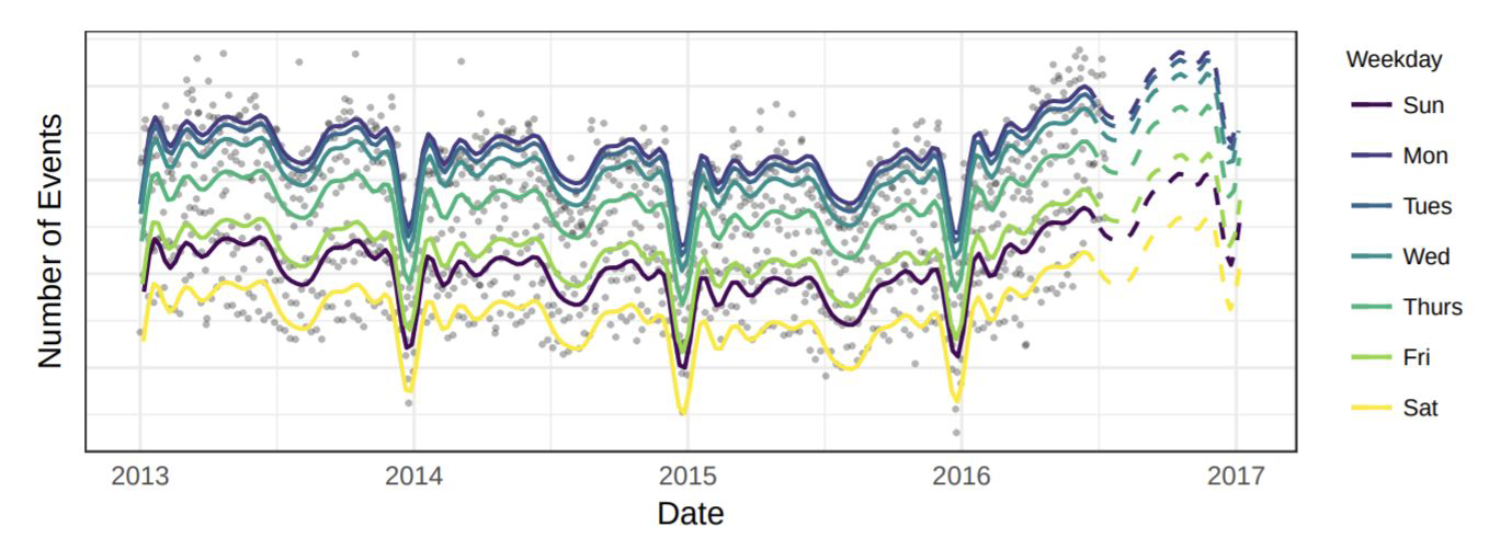
Facebook’s Prophet#
Harvey, A.C. and Peters, S. (1990), “Estimation Procedures for Structural Time Series Models” Taylor, S.J. and Letham, B. (2017), “Forecasting at Scale”
Library open-sourced for automated forecasting
Based on decomposable time series model
\(x_t = g(t) + s(t) + h(t) + \varepsilon_t\)
\(g(t)\) : trend function
\(s(t)\) : periodic changes
\(h(t)\) : holiday effects
Time is the only feature
several linear and non-linear functions of time
Needs not to be regularly spaced
Easily interpretable
Harvey, A.C. and Peters, S. (1990), “Estimation Procedures for Structural Time Series Models”
Taylor, S.J. and Letham, B. (2017), “Forecasting at Scale”
Rocket#
Open-source library for time classification
Uses CNN with >10.000 random convolutional filters
Then Logistic Regression
Exceptionally fast
1h 15min vs. 16h of alternative methods
Dempster, A. et al. (2019): “ROCKET: Exceptionally fast and accurate time series classification using random convolutional kernels”
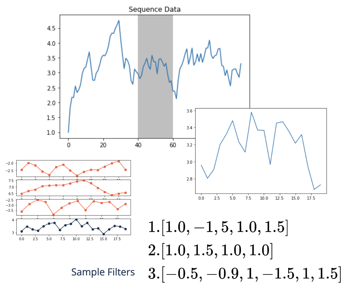
Convolutional neural networks#
As with images slide the kernel over the sequence data to detect patterns
If the data pattern matches the filter we see spikes
Later layers in CNNs respond to more complicated patterns, i.e. higher {specialization}
In 1D-convolutions we can use longer filters or add layers
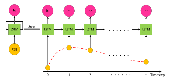
Long-Short-Term-Memory networks#
LSTMs are special network layers that carry memory for short-term and long-term information
Appropriateness ambiguous
Often do not beat exponential smoothing
Sometimes very good results
Very data hungry
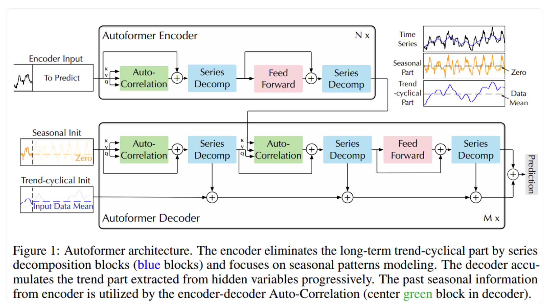
Transformer models#
A very promising model is autoformer
Good long-term predictions
Very data hungry, not much experience yet
Also, hard to predict when they will work well
Conclusion#
Many models - where to start#
As usual: with a good EDA
Find what is characteristic
Start with simple models
Exponential smoother are very good for forecasting
ARMA models are well interpretable and allow simulations and control
Only go to more complex or specific models, if you have to
and if your data amount allows you to
Resources#
Brockwell, P.J. and Davis, R.A. “Introduction to time series and forecasting”
Brockwell, P.J. and Davis, A.R. “Time Series Analysis”
Heij, C. et al., “Econometric Methods With Applications in Business and Economics”
https://machinelearningmastery.com/multi-step-time-series-forecasting/
ACF / PACF#
acf_pacf(df_acf_pacf)
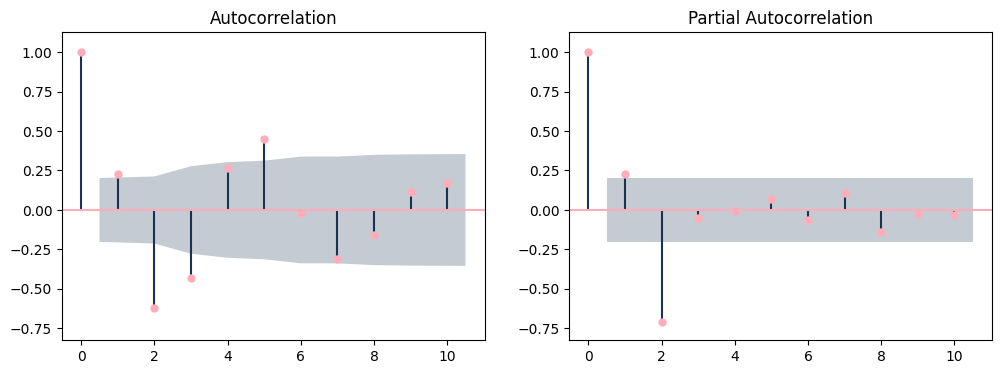
They all have 0/1 as a first value (auto correlation without lag. “what is the temperatur now compared with the temperatur now. wow the same, hence 1”) they have the same value for the first lag. After that, they differ.
ACF / PACF#
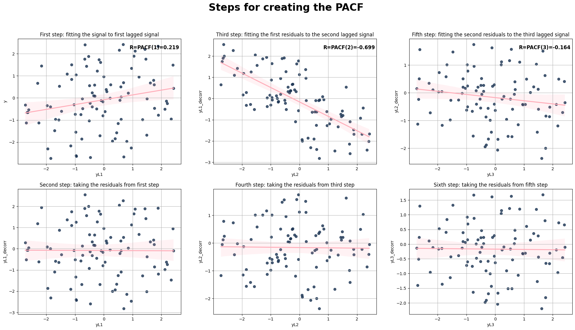
Step - by - step visualisation to aid explaining the difference between ACF and PACF. For PACF, in each step the stuff that was already explained by the shorter autocorrelations is removed.